| Input Datasets | |||
| Data sources for market baseline calculations (2022 seed, current subsidy) | |||
| Dataset | Records | Variables | Notes |
|---|---|---|---|
| Farmers (02_06_s22_sub00) | 7,429 | 165 | Per-farmer adoption scores, p_entry, profile |
| Model configuration (02_05) | — | — | 6 continuous params: floor_S=0.95, floor_M=0.5, floor_L=0.2, k_S=8, k_M=4, k_L=0.5 |
| Individuals (01_04) | 46,017 | 93 | Individual nutritional intake with survey weights |
| Travel time matrix (06_00) | 484 | 6 | 22x22 asymmetric OSRM travel time matrix |
| Source: ENCOVI 2023 (MAGA-calibrated), Module 2 outputs, OSRM (OpenStreetMap routing). | |||
Market Baseline Calculation
Module 6: Scenarios
Why Calculate a Market Baseline?
Scenario modeling requires establishing the supply-demand balance for white maize across Guatemala’s 22 departments. Before simulating biofortification production coverage scenarios, we must quantify:
- Production capacity — How much maize can each department produce if all farmers adopt biofortified varieties?
- Consumption demand — How much maize does each department’s population require?
- Structural surplus/deficit — Which departments produce more than they consume, and which face structural deficits?
This baseline enables realistic scenario projections that account for geographic heterogeneity in agricultural capacity and population density. It also feeds three structural elements that govern how production reaches consumption across the country: the continuous adoption curves that determine each farmer’s contribution, the production coverage scale that places each national production coverage level on the adoption ranking, and the gravity-based redistribution model that channels surplus from producing departments to deficit departments along real travel times.
The figures presented here correspond to the baseline scenario combining the 2022 biofortified seed variety with the current subsidy regime as of April 2026. Alternative seed variants and subsidy regimes are evaluated in the Shiny dashboard.
Data Integration
The market baseline integrates four data sources:
- Farmer adoption data (from Module 2) — Contains farmer rankings, production capacity, segment assignments, calibrated survey weights, and the per-farmer continuous adoption parameters (
p_entry,profile) that govern conversion intensity across production coverage levels. - Individual nutrient intake (from Module 1) — Contains population counts by department for consumption demand calculations.
- Calibrated model configuration (from Module 2) — Contains the six continuous adoption curve parameters (
floor_S/M/L,k_S/M/L) calibrated against empirical anchors. - Travel time matrix (from the one-shot routing script of this module) — Contains the 22×22 driving-time matrix between departmental capitals and the derived gravity weights.
The farmer dataset contains expanded records (from MAGA weight calibration (Ministerio de Agricultura, Ganadería y Alimentación, 2023)) with adoption priority scores and the continuous adoption parameters per farmer, while the individual dataset provides the population base for consumption calculations. The model configuration provides the six scalar parameters that define the sigmoid conversion curves used downstream.
Departmental Baseline Metrics
All calculations use survey weights to produce population-representative estimates. The baseline captures four dimensions for each department: farmer population by technology segment, land area allocation, annual consumption demand, and production capacity (current and maximum biofortified).
NoteConsumption Reference Values
Two consumption benchmarks inform our analysis:
- Direct human consumption: 110 kg/capita/year — Lower-bound estimate for direct food use only (primarily tortillas).
- FSI consumption: 174 kg/capita/year — Includes food, seed retention, animal feed, and post-harvest losses.
Consumption coverage calculations use the FSI estimate (USDA Foreign Agricultural Service, 2019) as the denominator, rather than direct human consumption (Ministerio de Agricultura, Ganadería y Alimentación, 2008), since biofortified production must satisfy total domestic demand.
Conversion factors used in the baseline:
- Kilograms to quintales: ÷ 45.36 (1 qq = 100 lb = 45.36 kg)
- Quintales to metric tons: × 0.04536 (1 qq ≈ 0.04536 MT)
- Manzanas to hectares: × 0.7 (1 mz = 0.7 ha)
| Departmental Market Baseline Metrics | ||||||||||
| Farmers, land, consumption, and production capacity by department | ||||||||||
| Department | Total Farmers | Hybrid Farmers | Non-hybrid Farmers | Land (ha) | Human Cons. (MT/yr) | FSI Cons. (MT/yr) | Current Prod. (MT) | Max Bio Prod. (MT) | Max Coverage (%) | |
|---|---|---|---|---|---|---|---|---|---|---|
| Guatemala | 19,316 | 314 | 19,002 | 20,257.6 | 367,944.1 | 582,020.6 | 37,049.1 | 42,243.4 | 7.3% | |
| El Progreso | 5,848 | 1,443 | 4,405 | 14,198.4 | 22,449.1 | 35,510.4 | 16,651.1 | 20,450.8 | 57.6% | |
| Sacatepéquez | 5,759 | 1,293 | 4,466 | 8,746.4 | 42,058.9 | 66,529.6 | 14,601.2 | 18,603.1 | 28.0% | |
| Chimaltenango | 46,641 | 12,142 | 34,499 | 24,384.7 | 83,299.0 | 131,763.9 | 48,320.4 | 60,009.1 | 45.5% | |
| Escuintla | 18,216 | 9,108 | 9,108 | 7,151.5 | 90,250.2 | 142,759.3 | 23,987.6 | 23,006.9 | 16.1% | |
| Santa Rosa | 37,379 | 16,335 | 21,043 | 16,149.5 | 49,575.8 | 78,419.9 | 40,210.0 | 44,477.4 | 56.7% | |
| Sololá | 9,459 | 2,463 | 6,997 | 17,184.8 | 49,054.4 | 77,595.1 | 36,763.5 | 47,485.1 | 61.2% | |
| Totonicapán | 19,718 | 3,344 | 16,374 | 29,563.7 | 54,423.5 | 86,088.1 | 45,321.0 | 59,007.5 | 68.5% | |
| Quetzaltenango | 25,551 | 5,289 | 20,262 | 43,607.2 | 94,319.1 | 149,195.6 | 117,061.0 | 149,819.2 | 100.0% | |
| Suchitepéquez | 13,115 | 5,122 | 7,993 | 8,182.6 | 65,358.7 | 103,385.6 | 25,183.0 | 28,647.1 | 27.7% | |
| Retalhuleu | 10,577 | 4,512 | 6,065 | 20,542.1 | 44,278.1 | 70,039.9 | 51,225.1 | 57,172.8 | 81.6% | |
| San Marcos | 54,490 | 12,403 | 42,087 | 52,370.3 | 133,230.2 | 210,746.0 | 115,168.8 | 149,205.5 | 70.8% | |
| Huehuetenango | 82,011 | 25,517 | 56,494 | 109,568.2 | 161,586.4 | 255,600.3 | 182,515.2 | 214,062.5 | 83.7% | |
| Quiché | 86,830 | 19,467 | 67,362 | 157,304.0 | 137,335.7 | 217,240.0 | 234,588.4 | 301,091.4 | 100.0% | |
| Baja Verapaz | 17,846 | 2,511 | 15,335 | 28,163.3 | 40,232.9 | 63,641.2 | 32,683.8 | 42,466.9 | 66.7% | |
| Alta Verapaz | 106,782 | 19,081 | 87,701 | 177,085.2 | 154,746.6 | 244,780.9 | 240,255.3 | 305,955.8 | 100.0% | |
| Petén | 42,446 | 9,241 | 33,205 | 249,562.6 | 62,040.1 | 98,136.2 | 483,453.3 | 592,053.7 | 100.0% | |
| Izabal | 37,863 | 11,178 | 26,685 | 21,081.0 | 53,807.8 | 85,114.2 | 56,915.6 | 64,666.2 | 76.0% | |
| Zacapa | 16,478 | 3,438 | 13,040 | 16,628.8 | 31,276.2 | 49,473.2 | 35,114.5 | 44,269.4 | 89.5% | |
| Chiquimula | 50,738 | 7,498 | 43,240 | 46,001.9 | 52,439.9 | 82,950.3 | 68,894.7 | 86,320.4 | 100.0% | |
| Jalapa | 21,668 | 2,807 | 18,861 | 28,209.9 | 44,635.6 | 70,605.4 | 49,675.7 | 64,366.3 | 91.2% | |
| Jutiapa | 54,742 | 14,157 | 40,585 | 60,268.9 | 61,735.3 | 97,654.0 | 120,057.7 | 147,643.1 | 100.0% | |
| Total | — | 783,474 | 188,662 | 594,812 | 1,156,213 | 1,896,077 | 2,999,250 | 2,075,696 | 2,563,024 | — |
| Source: ENCOVI 2023 (MAGA-calibrated). Human Cons. = 110 kg/capita/year (lower-bound estimate). FSI Cons. = 174 kg/capita/year (USDA 2019). Green = surplus (≥100%). Red = deficit (<50%). Production capacity shares cited in the text (e.g., a department's share of national production) are relative to the national total; consumption coverage and surplus/deficit status are relative to each department's own annual FSI consumption demand. | ||||||||||
The baseline is geographically concentrated. Petén alone accounts for 23.1% of national maize production capacity, and together with Alta Verapaz and Quiché for 46.8%, while Guatemala department, the most populous, covers 7.3% of its own FSI demand from local production. Six departments (highlighted in green) reach or exceed 100% consumption coverage from local production alone; five (highlighted in red) stay below 50% even at full production coverage.
ImportantStructural Supply-Demand Imbalance
Even at 100% biofortified production coverage, 6 of the 22 departments satisfy their local consumption demand from their own production. The other 16 range from 7.3% to 91.2% coverage. This is what the redistribution model that follows is built for: without surplus moving between departments, a national consumption coverage target cannot be met from a geographically concentrated supply.
Continuous Adoption Model
Adoption is implemented as a continuous process rather than a binary admit / exclude rule. Each farmer carries two attributes calibrated in Module 2:
- A per-farmer entry point
p_entry— the farmer’s position on the national adoption ranking. Farmers are ordered by adoption score and the ranking is scaled by cumulative maize production, sop_entryruns from 0 for the first farmer to 1. - A behavioural profile
S,M, orL(Small, Medium, Large entry-size) — that governs the steepness of conversion intensity from the entry point onwards.
Farmer-level adoption is evaluated at an internal adoption index p_internal, measured on the same ranking scale. Every farmer with p_entry ≤ p_internal is in the adoption pool. The fraction of that farmer’s maize land, and of their potential biofortified production, converted at p_internal is the conversion ratio:
\[ r_i(p_{internal}) = \text{sigmoid}(p_{internal}, p_{entry,i}, \text{floor}_{profile}, k_{profile}) \]
where floor_{profile} is the conversion fraction at the entry point itself, and k_{profile} controls how rapidly conversion rises from the floor towards 1 as p_internal increases. The six scalar parameters (floor_S, floor_M, floor_L, k_S, k_M, k_L) come from the model configuration calibrated in Module 2 against empirical adoption anchors via median absolute deviation. At p_internal = 0 no farmer is in the pool; at p_internal = 1 every farmer is in the pool with r_i(1) = 1 by construction.
The effective biofortified production of farmer i at internal adoption index p_internal is therefore:
\[ \text{bio}_i(p_{internal}) = \text{production\_biofortified}_i \times \text{weight\_calibrated}_i \times r_i(p_{internal}) \]
This formulation captures realistic adoption patterns where early adopters are not uniformly distributed across departments, and where each farmer’s conversion intensity varies by behavioural profile and position along the adoption ranking. It also produces smooth saturation trajectories (shown in the consumption coverage analysis below) that converge to the maximum biofortified production capacity at full production coverage.
The internal adoption index records a position on a ranking scaled by production; production coverage records how much maize-growing area is planted with biofortified seed. The next section builds the scale that connects the two.
Production Coverage Scale
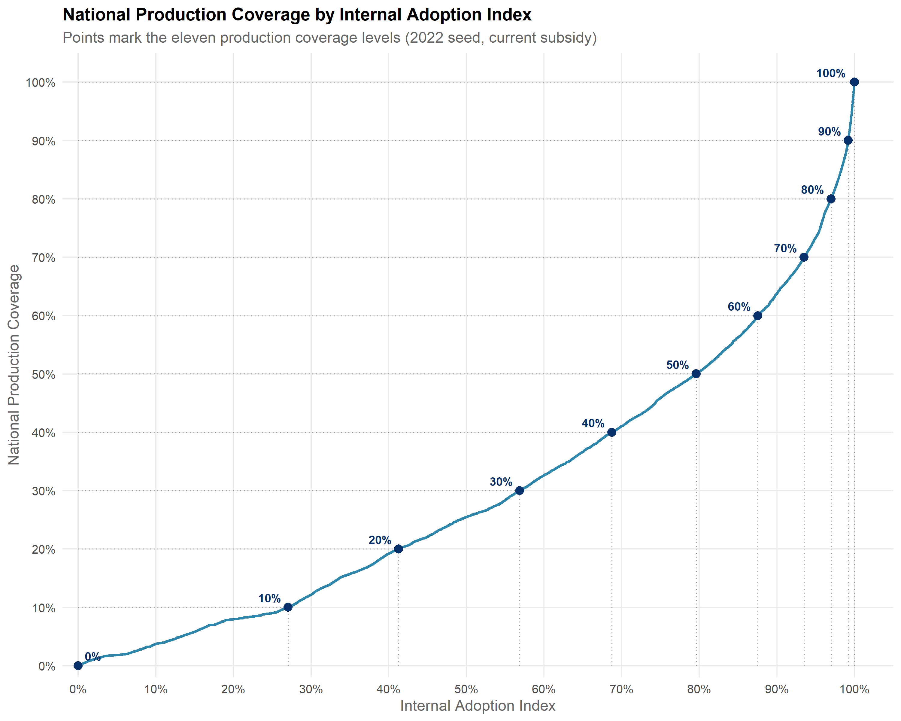
The scenarios are defined on production coverage, the share of maize-growing area planted with biofortified seed, at eleven levels from 0% to 100% in steps of 10 percentage points. Each production coverage level is evaluated at the internal adoption index that plants that share of maize land with biofortified seed. The association is computed separately for each seed variant and subsidy regime, since both shape the adoption ranking.
The framework evaluates the internal adoption index on a grid of 10,001 equally spaced values between 0 and 1. At each value, national production coverage is the converted maize land over the total maize land:
\[ \text{production coverage}(p_{internal}) = \frac{\sum_i \text{land\_wtcorn}_i \times r_i(p_{internal}) \times \text{weight\_calibrated}_i}{\sum_i \text{land\_wtcorn}_i \times \text{weight\_calibrated}_i} \]
Numerator and denominator share the same land unit, so the ratio needs no conversion. Each of the eleven levels is assigned the grid value whose production coverage is closest to its target, and the two endpoints are fixed: 0% corresponds to an empty adoption pool and 100% to full adoption, where every farmer has r_i(1) = 1.
The association error does not exceed 0.013 percentage points at any level. Reaching 10% production coverage takes the ranking to an internal adoption index of 0.27, and reaching 50% takes it to 0.8: farmers enter the adoption pool at their profile floor and convert the rest of their land only as the index advances.
NoteReading the Scenario Levels
Every result reported by production coverage level, in this module and in the dashboard, refers to the share of maize-growing area planted with biofortified seed. The internal adoption index stays inside the calculation: it selects the adopting farmers and their conversion ratios, and it is not reported as a scenario level.
Consumption Coverage Before Redistribution
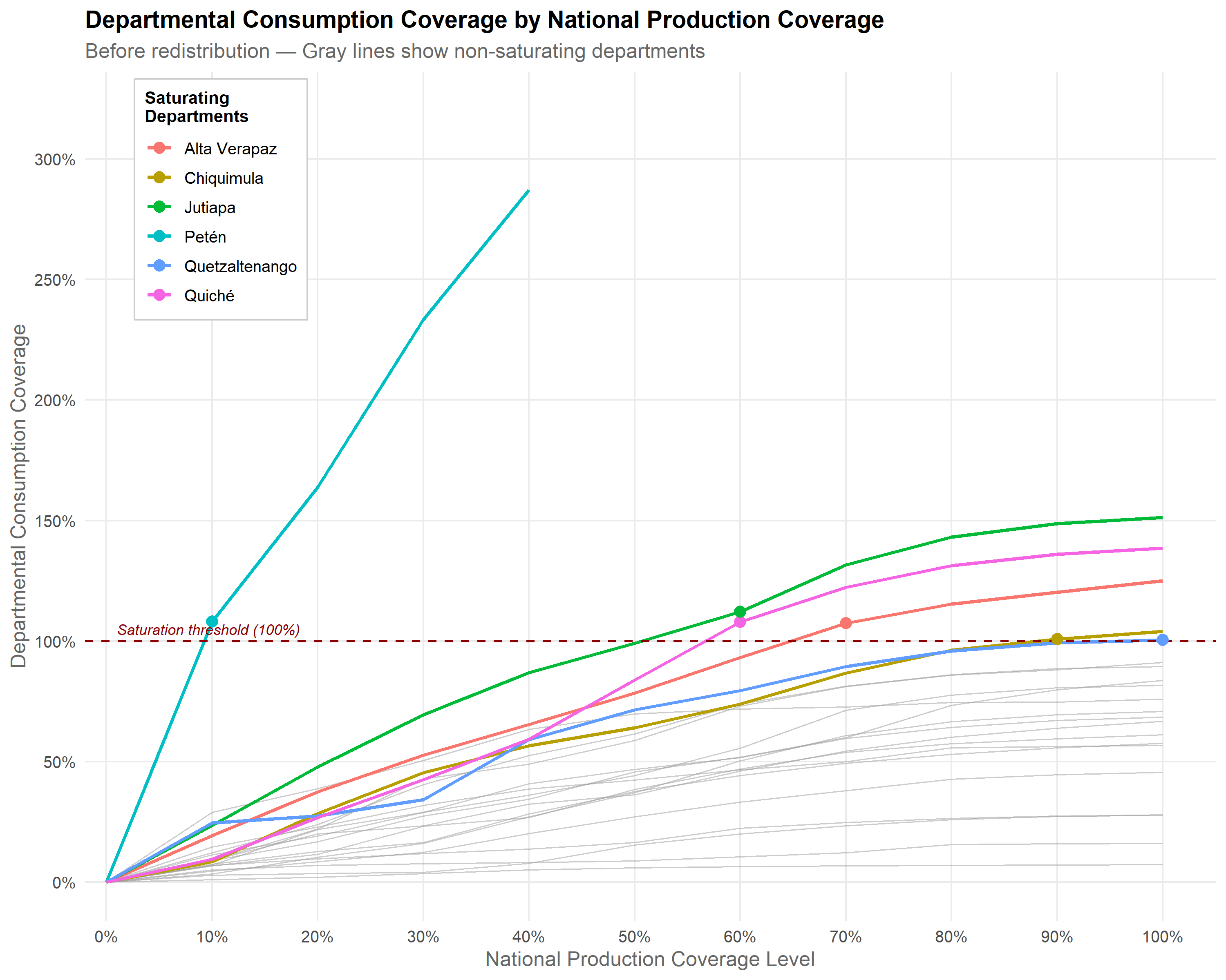
Before introducing inter-departmental redistribution, we analyse how departmental consumption coverage evolves across the national production coverage range (0–100%) based solely on local production. At each production coverage level, the biofortified production realised in department d is the sum of bio_i(p_internal) across all farmers i located in d, evaluated at the internal adoption index associated with that level. Coverage is the ratio between this realised production and the department’s annual FSI consumption demand.
This analysis surfaces the departments that saturate early (reach 100% local coverage at low national production coverage) — these are the natural supply nodes for the redistribution model that follows.
NoteSaturation Timing
Departments that reach 100% consumption coverage at lower national production coverage levels have production capacity that exceeds local demand. These early saturators become natural supply nodes for the redistribution model: once their own demand is satisfied, additional biofortified production from local farmers is available to supply deficit departments elsewhere in the country.
Travel Time Infrastructure
Redistribution between Guatemalan departments is not symmetric in space. The country’s road network is shaped by mountain ranges (Sierra Madre, Sierra de los Cuchumatanes) that create significant travel time asymmetries between departments that are geographically close but poorly connected by road. The gravity-based redistribution model therefore uses real driving times rather than Euclidean distances or simple adjacency.
The 22×22 travel time matrix between departmental capitals is computed once, by a separate one-shot routing script. That script queries the Open Source Routing Machine (OSRM) over OpenStreetMap road network data and produces a deterministic matrix that depends only on the road network. The matrix is stored as a parquet file and re-used across all seed × subsidy combinations of the scenario pipeline.
Departmental Capitals
The reference points for the travel time matrix are the administrative seats (cabeceras departamentales) of each of Guatemala’s 22 departments, as defined by Guatemala’s Instituto Nacional de Estadística (INE). Coordinates were obtained from the GeoNames geographical database (https://www.geonames.org, Creative Commons Attribution 4.0 License), which aggregates data from official national mapping agencies and the OpenStreetMap community. Each coordinate corresponds to the populated place record classified as feature class P (populated place) and feature code PPLA (seat of a first-order administrative division) in GeoNames. Coordinates are in WGS84 (EPSG:4326).
| Departmental Capitals of Guatemala | |||
| Reference points for OSRM travel time computation | |||
| Department | Capital (Cabecera) | Latitude | Longitude |
|---|---|---|---|
| Guatemala | Guatemala City | 14.6349 | −90.5069 |
| El Progreso | Guastatoya | 14.8536 | −90.0672 |
| Sacatepéquez | Antigua Guatemala | 14.5586 | −90.7295 |
| Chimaltenango | Chimaltenango | 14.6619 | −90.8193 |
| Escuintla | Escuintla | 14.2980 | −90.7870 |
| Santa Rosa | Cuilapa | 14.2765 | −90.2984 |
| Sololá | Sololá | 14.7725 | −91.1866 |
| Totonicapán | Totonicapán | 14.9082 | −91.3607 |
| Quetzaltenango | Quetzaltenango | 14.8347 | −91.5183 |
| Suchitepéquez | Mazatenango | 14.5336 | −91.5037 |
| Retalhuleu | Retalhuleu | 14.5340 | −91.6781 |
| San Marcos | San Marcos | 14.9647 | −91.7963 |
| Huehuetenango | Huehuetenango | 15.3195 | −91.4714 |
| Quiché | Santa Cruz del Quiché | 15.0295 | −91.1502 |
| Baja Verapaz | Salamá | 15.1025 | −90.3160 |
| Alta Verapaz | Cobán | 15.4713 | −90.3707 |
| Petén | Flores | 16.9316 | −89.8923 |
| Izabal | Puerto Barrios | 15.7280 | −88.5940 |
| Zacapa | Zacapa | 14.9719 | −89.5294 |
| Chiquimula | Chiquimula | 14.7979 | −89.5449 |
| Jalapa | Jalapa | 14.6354 | −89.9889 |
| Jutiapa | Jutiapa | 14.2916 | −89.8953 |
| Source: GeoNames geographical database (https://www.geonames.org, CC BY 4.0). Coordinates in WGS84 (EPSG:4326). | |||
Travel Time Matrix
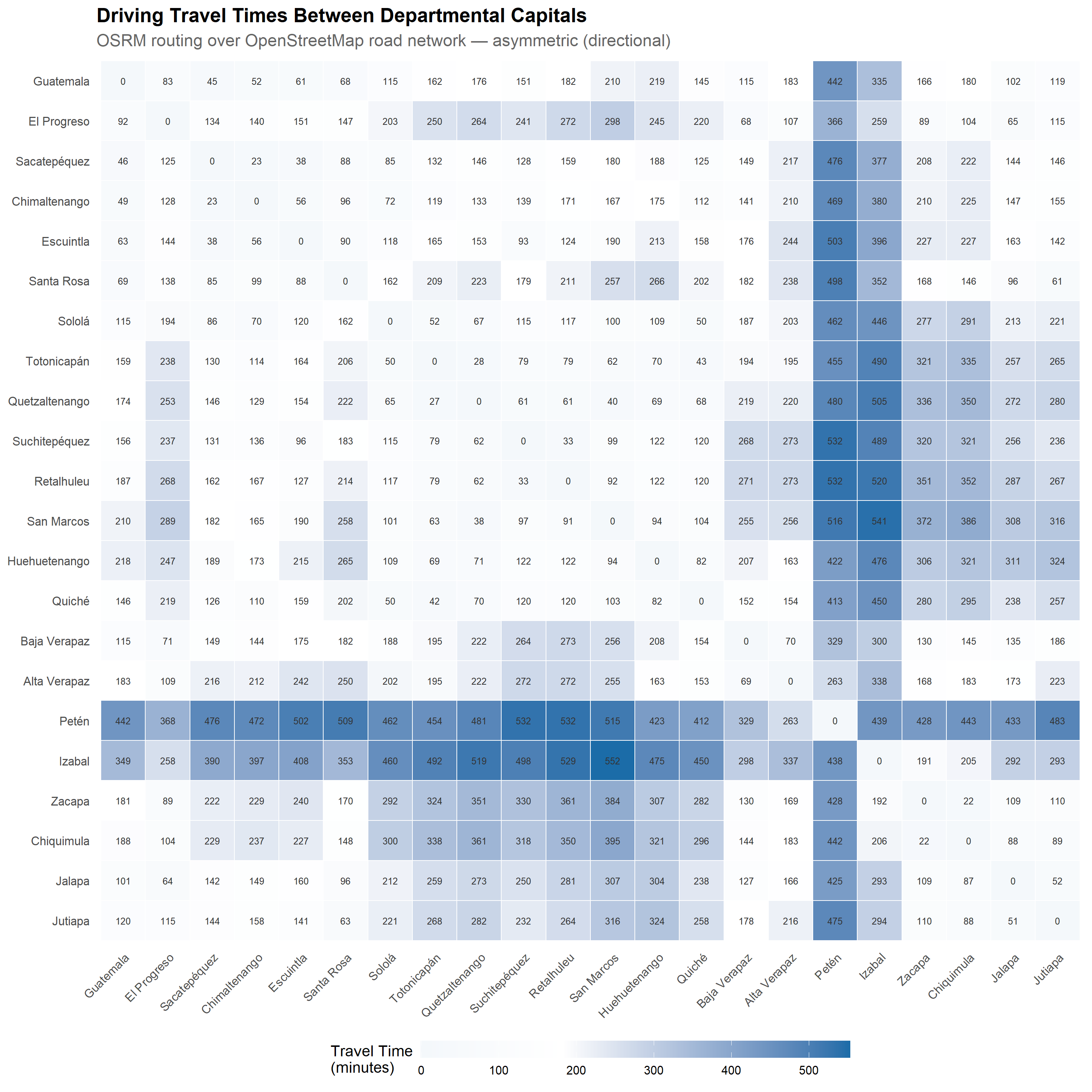
The matrix below shows driving times in minutes between every pair of departmental capitals. The matrix is asymmetric — t(i, j) ≠ t(j, i) in general — reflecting real directional differences in road routing, terrain gradients, and directional constraints in Guatemala’s road network.
Gravity Weights
From the travel time matrix we derive a matrix of gravity weights w(i, j) = 1 / travel_time(i, j)^β, with a decay parameter β = 2, the Newtonian specification used in the trade gravity literature (Anderson & van Wincoop, 2003). The summary below characterises the resulting weight distribution over the 462 ordered department pairs, whose driving times run from 21.6 to 552.5 minutes.
| Gravity Weight Matrix Summary | |
| w(i,j) = 1 / travel_time(i,j)² — Anderson & van Wincoop (2003) | |
| Metric | Value |
|---|---|
| Beta (decay parameter) | 2 |
| Number of department pairs | 462 |
| Min gravity weight | 3.28e-06 |
| Max gravity weight | 2.14e-03 |
| Mean gravity weight | 9.13e-05 |
| Min travel time (min) | 21.6 |
| Max travel time (min) | 552.5 |
| Mean travel time (min) | 215.2 |
| Source: OSRM travel time matrix. Statistics computed over off-diagonal pairs (origin ≠ destination). | |
Gravity-Based Redistribution Model
The redistribution model channels surplus biofortified production from departments that exceed their local demand to departments that face a deficit. The flow allocation follows the gravity formulation of (Anderson & van Wincoop, 2003), adapted here to inter-departmental commodity movement within Guatemala. The model is implemented in the utility function redistribute_gravity() of the framework’s centralized function file.
For each donor department i with surplus production S_i and each receiver department j with deficit D_j, the share of S_i that flows to j is proportional to:
\[ \text{flow}_{i \to j} \;\propto\; D_j \;\times\; w(i, j) \]
where w(i, j) = 1 / travel_time(i, j)² is the gravity weight defined above. The proportionality gives the allocation two structural properties: receivers with larger deficits attract a larger share of surplus, the demand pull, and receivers further away by road attract a smaller share, the distance friction. Flows are normalised so that the total volume out of i equals S_i. The asymmetric travel time matrix means the flow i → j may differ from j → i, which matters when topographic asymmetry makes one direction more accessible than the other.
The gravity model uses real driving times rather than nominal adjacency, captures the terrain effects that adjacency hides, and evaluates all donor-receiver pairs jointly without requiring an external ordering rule.
Production Conservation
A direct consequence of the proportional allocation is that total biofortified production is conserved through redistribution: the volume leaving each donor equals the volume distributed across receivers. The check below evaluates this at full national production coverage, the most demanding case, where every department is simultaneously active in the redistribution network.
| Production Conservation Check | |
| Validation at 100% national production coverage — gravity redistribution | |
| Metric | Value |
|---|---|
| Total bio production before redistribution (qq) | 56,504,051 |
| Total bio production after redistribution — capped (qq) | 56,504,051 |
| Remaining excess after redistribution (qq) | 0 |
| Total accounted (capped + excess) (qq) | 56,504,051 |
| Difference (loss/gain) (qq) | 0 |
| Difference as % of total production | 0% |
| A non-zero difference indicates production loss or creation through redistribution. Values near zero (< 1 qq) are acceptable due to floating-point arithmetic. | |
Consumption Coverage After Redistribution
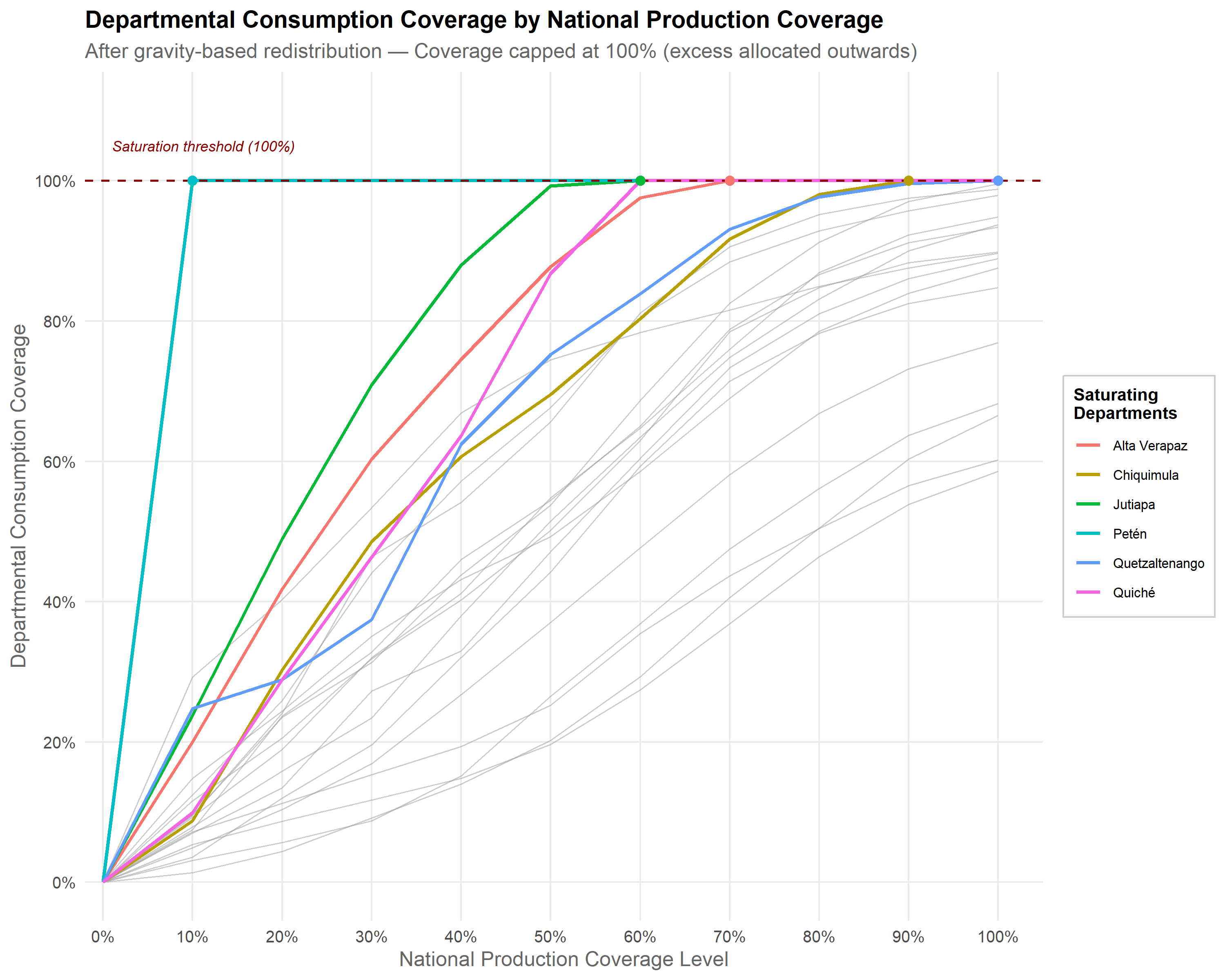
With the gravity model applied, departmental consumption coverage at each production coverage level reflects both local production (from the continuous adoption curves) and received flows from surplus departments (from the gravity allocation). The two outputs below summarise the post-redistribution market structure: the saturation order describes how progressively more departments reach 100% local coverage as national production coverage rises, and the saturation curves describe the smoothed trajectories for every department.
Saturation Order
The table below ranks departments by the national production coverage level at which each first reaches 100% consumption coverage after gravity redistribution. Departments that do not reach saturation even at 100% national production coverage are marked with “—”, indicating insufficient inflow through the gravity network to close their local deficit.
| Departmental Saturation Order | ||
| Production coverage level at which each department reaches 100% coverage (after gravity redistribution) | ||
| Order | Department | Saturation Point |
|---|---|---|
| 1 | Petén | 10% |
| 2 | Jutiapa | 60% |
| 3 | Quiché | 60% |
| 4 | Alta Verapaz | 70% |
| 5 | Chiquimula | 90% |
| 6 | Quetzaltenango | 100% |
| — | Baja Verapaz | — |
| — | Chimaltenango | — |
| — | El Progreso | — |
| — | Escuintla | — |
| — | Guatemala | — |
| — | Huehuetenango | — |
| — | Izabal | — |
| — | Jalapa | — |
| — | Retalhuleu | — |
| — | Sacatepéquez | — |
| — | San Marcos | — |
| — | Santa Rosa | — |
| — | Sololá | — |
| — | Suchitepéquez | — |
| — | Totonicapán | — |
| — | Zacapa | — |
| Saturation point = national production coverage level at which the department first reaches 100% local consumption coverage post-redistribution. A dash indicates the department does not saturate even at 100% national production coverage. | ||
Saturation Curves
The figure below shows the post-redistribution consumption coverage trajectory for every department across the full production coverage range. Compared with the pre-redistribution curves shown earlier, the gravity model raises the deficit departments as national production coverage grows, and caps the apparent surplus of donor departments at 100%, since their excess beyond local demand has been allocated outwards. At full production coverage the lowest departmental coverage rises to 58.6%, and the largest single gain is 59.3 percentage points in Guatemala, which moves from 7.3% to 66.5%.
Market Metrics After Redistribution
The final table consolidates the market-level outcomes at full national production coverage, comparing pre- and post-redistribution coverage to quantify the contribution of the gravity model to closing departmental deficits.
| Market Structure: Pre vs Post Redistribution | |||||||
| Comparison at 100% national production coverage | |||||||
| departamento | n_farmers_total | land_ha_total | max_bio_production_mt | max_coverage_before | bio_production_after_mt | coverage_after | coverage_change |
|---|---|---|---|---|---|---|---|
| Guatemala | 19316 | 20258 | 42243 | 7.258 | 387198 | 66.53 | 59.268 |
| El Progreso | 5848 | 14198 | 20451 | 57.591 | 33281 | 93.72 | 36.130 |
| Sacatepéquez | 5759 | 8746 | 18603 | 27.962 | 45406 | 68.25 | 40.287 |
| Chimaltenango | 46641 | 24385 | 60009 | 45.543 | 101335 | 76.91 | 31.364 |
| Escuintla | 18216 | 7152 | 23007 | 16.116 | 83643 | 58.59 | 42.474 |
| Santa Rosa | 37379 | 16150 | 44477 | 56.717 | 68666 | 87.56 | 30.846 |
| Sololá | 9459 | 17185 | 47485 | 61.196 | 68993 | 88.91 | 27.718 |
| Totonicapán | 19718 | 29564 | 59008 | 68.543 | 80397 | 93.39 | 24.846 |
| Quetzaltenango | 25551 | 43607 | 149819 | 100.000 | 149196 | 100.00 | 0.000 |
| Suchitepéquez | 13115 | 8183 | 28647 | 27.709 | 62253 | 60.21 | 32.505 |
| Retalhuleu | 10577 | 20542 | 57173 | 81.629 | 62909 | 89.82 | 8.189 |
| San Marcos | 54490 | 52370 | 149206 | 70.799 | 178667 | 84.78 | 13.980 |
| Huehuetenango | 82011 | 109568 | 214063 | 83.749 | 242435 | 94.85 | 11.100 |
| Quiché | 86830 | 157304 | 301091 | 100.000 | 217240 | 100.00 | 0.000 |
| Baja Verapaz | 17846 | 28163 | 42467 | 66.729 | 63345 | 99.53 | 32.806 |
| Alta Verapaz | 106782 | 177085 | 305956 | 100.000 | 244781 | 100.00 | 0.000 |
| Petén | 42446 | 249563 | 592054 | 100.000 | 98136 | 100.00 | 0.000 |
| Izabal | 37863 | 21081 | 64666 | 75.976 | 76301 | 89.65 | 13.670 |
| Zacapa | 16478 | 16629 | 44269 | 89.481 | 48459 | 97.95 | 8.469 |
| Chiquimula | 50738 | 46002 | 86320 | 100.000 | 82950 | 100.00 | 0.000 |
| Jalapa | 21668 | 28210 | 64366 | 91.163 | 69779 | 98.83 | 7.667 |
| Jutiapa | 54742 | 60269 | 147643 | 100.000 | 97654 | 100.00 | 0.000 |
| Pre-redistribution metrics rely solely on local production at 100% production coverage. Post-redistribution metrics incorporate gravity-weighted flows from surplus departments to deficit departments. | |||||||
Summary
Baseline Framework
The market baseline characterises the supply-demand structure of white maize across Guatemala’s 22 departments and supplies four structural elements consumed downstream by the scenario precomputation step:
- Per-department baseline metrics — Farmer counts by segment, land area, FSI consumption demand, current production, and maximum biofortified production capacity.
- Continuous adoption parameters — The six scalar parameters (
floor_S/M/L,k_S/M/L) calibrated in Module 2 that define the per-farmer conversion ratio along the adoption ranking. - Production coverage scale — The internal adoption index at which each of the eleven production coverage levels is evaluated, specific to each seed variant and subsidy regime.
- Gravity redistribution infrastructure — The 22×22 OSRM travel time matrix and the derived gravity weights that channel surplus from donor departments to deficit departments.
Key Findings
Structural geographic heterogeneity — Petén concentrates nearly a quarter of national maize production capacity, while several densely populated departments face structural deficits below 50% of FSI demand even at full local production. This heterogeneity makes inter-departmental redistribution a necessary component of any national consumption coverage target.
Production coverage is measured on maize land — Farmers enter the adoption pool at their profile floor and convert the rest of their land progressively, so each intermediate production coverage level sits further along the adoption ranking than its nominal value: 50% of maize land corresponds to an internal adoption index of 0.8. Every scenario level is evaluated at its associated index, with an association error of at most 0.013 percentage points.
Gravity redistribution narrows deficits without creating production — The Anderson & van Wincoop formulation channels surplus to deficit departments along real driving times. At full production coverage the lowest departmental coverage rises from 7.3% to 58.6%, while the number of departments reaching 100% stays at 6: the model closes the distance to saturation without adding saturating departments. Total production before and after redistribution matches to 0 qq.
Travel time asymmetry — Inter-departmental driving times run from 21.6 to 552.5 minutes across 462 ordered pairs, and differ by direction. The asymmetric matrix returned by OSRM carries that structure, which a symmetric distance or a simple adjacency rule would not.
Application
The outputs of this script feed the scenario precomputation step, which uses the per-department coverage trajectories to assign biofortified maize consumption to children via the hierarchical priority assignment, and then aggregates the resulting individual nutrient and stunting outcomes at departmental and national level.
Limitations
- Driving mode only — The travel time matrix assumes road transport. Alternative routes (river, air) are not modelled.
- Static road network — Travel times reflect the OSM road network at the time of OSRM computation. Major infrastructure changes such as new highways or bridge construction would require the routing script to be run again.
- Single reference point per department — Travel times are measured between cabeceras departamentales. Intra-departmental distribution costs are not modelled.
- No seasonal variation — Travel times do not account for seasonal road conditions (rainy season closures, flooding).
References
Anderson, J. E., & van Wincoop, E. (2003). Gravity with gravitas: A solution to the border puzzle. American Economic Review, 93(1), 170–192. https://doi.org/10.1257/000282803321455214
Ministerio de Agricultura, Ganadería y Alimentación. (2008). Segundo Informe Nacional sobre el Estado de los Recursos Fitogenéticos de Guatemala. MAGA/UNR.
Ministerio de Agricultura, Ganadería y Alimentación. (2023). Informe de Producción de Granos Básicos. MAGA/DIPLAN.
USDA Foreign Agricultural Service. (2019). Guatemala: Grain and Feed Annual (GAIN Report No. GT19007). USDA Foreign Agricultural Service.