Likely Adopters Model Calibration

Module 2: Economic Impact

Why Calibrate a Likely Adopters Model?

The economic impact of biofortified maize depends on which farmers adopt, not only on how much each adopter benefits. Without a model of the adoption process, every farmer would have to be treated as equally likely to adopt, against the empirical evidence that Semilla Nueva’s market composition at every observed production coverage level is concentrated in specific farmer profiles.

The Likely Adopters model assigns each farmer a composite score reflecting their expected priority for adoption, and a continuous adoption ratio reflecting the fraction of their white-maize land that they would commit to biofortified seed at any given national production coverage level. The model is calibrated rather than fit: its structural parameters are tuned to reproduce five empirical anchors provided by Semilla Nueva (per-segment cohort composition at production coverage levels 5%, 10%, 20%, 30%) plus one structural anchor (population composition at 100% production coverage).

This module documents the determination of the model parameters: variable selection (Phase A–C), construction of the calibration anchor set (Phase D), and sequential sensitivity sweeps over the architectural components of the scoring engine (Phase E), the risk-aversion penalty (Phase F), and the continuous-adoption curve (Phase G). The final consolidated configuration is summarised in the integrated evaluation section and consumed downstream when applying the model.

The figures presented here correspond to the baseline scenario combining the 2022 biofortified seed variety with the current subsidy regime. The structural parameters identified depend on the joint distribution of farmer characteristics, not on the magnitude of the projected economic benefit; a single calibration on the baseline therefore produces the model configuration applicable across all seed × subsidy combinations evaluated downstream.

Phase A — B — C: Variable Selection

The selection pipeline operates on the joined economic impact and segmentation dataset for the baseline configuration. Three complementary filters reduce the candidate set to a small group of predictors with demonstrated statistical association with adoption priority:

Correlation filter — discards numeric variables with a correlation above 0.80 against another retained variable.
Near-zero variance filter — discards variables with frequency ratio above 19 and percent unique below 10%, indicating insufficient variation to support prediction.
Boruta feature selection — applies the Boruta algorithm (Random Forest importance against shadow-permuted variables) to identify variables with statistically significant association with an adoption priority proxy.

The adoption priority proxy is a five-level ordinal score derived from segment positioning and projected income increment, reflecting Semilla Nueva’s strategic targeting logic.

Correlation Filter

Highly correlated variables provide redundant information; the algorithm retains one and discards the other based on mean absolute correlation against the rest of the candidate set.

Table 1: Variables Removed Due to High Correlation (r > 0.80)

Variables Removed: High Correlation Filter. 27 of 81 numeric variables removed (cutoff r = 0.80)
Variable Removed	Reason
Variables Removed: High Correlation Filter
27 of 81 numeric variables removed (cutoff r = 0.80)
cost_total_current	Correlation > 0.80 with retained variable
exp_total	Correlation > 0.80 with retained variable
cost_non_seed	Correlation > 0.80 with retained variable
exp_non_seed	Correlation > 0.80 with retained variable
value_total_economic	Correlation > 0.80 with retained variable
land_wtcorn_annual	Correlation > 0.80 with retained variable
revenue	Correlation > 0.80 with retained variable
income_sales	Correlation > 0.80 with retained variable
exp_fertilizers	Correlation > 0.80 with retained variable
sale_share	Correlation > 0.80 with retained variable
value_gross	Correlation > 0.80 with retained variable
net_position_qq	Correlation > 0.80 with retained variable
pct_sold	Correlation > 0.80 with retained variable
income_net_current	Correlation > 0.80 with retained variable
total_production	Correlation > 0.80 with retained variable
n_harvests_total	Correlation > 0.80 with retained variable
exp_seeds_per_mz	Correlation > 0.80 with retained variable
qty_retained_qq	Correlation > 0.80 with retained variable
value_self_consumption_total	Correlation > 0.80 with retained variable
value_self_consumption	Correlation > 0.80 with retained variable
exp_total_per_mz	Correlation > 0.80 with retained variable
exp_non_seed_per_mz	Correlation > 0.80 with retained variable
exp_total_per_mz_annual	Correlation > 0.80 with retained variable
exp_seeds_per_mz_annual	Correlation > 0.80 with retained variable
pobreza	Correlation > 0.80 with retained variable
yield_zscore_dept	Correlation > 0.80 with retained variable
yield_wtcorn_annual	Correlation > 0.80 with retained variable
Selection via caret::findCorrelation (removes variable with highest mean absolute correlation).

Near-Zero Variance Analysis

The framework reports the variance diagnostic for the variables that survive the correlation filter. Variables with extremely concentrated distributions provide little signal regardless of statistical importance and are removed before Boruta evaluation.

Table 2: Near-Zero Variance Analysis for Post-Correlation Variables

Near-Zero Variance Analysis. Predictor variables with potentially insufficient variation
Variable	Frequency Ratio¹	% Unique Values²	NZV Flag³
Near-Zero Variance Analysis
Predictor variables with potentially insufficient variation
land_wtcorn	1.171	8,274.33%	FALSE
yield_wtcorn_qq	1.078	8,635.08%	FALSE
farmer_age	1.030	8,487.01%	FALSE
farmer_male	7.834	2.69%	FALSE
farmer_ed	1.807	9.42%	FALSE
qty_sold_qq	149.500	5,397.77%	FALSE
qty_household_qq	7.500	8,668.73%	FALSE
qty_animal_seed_qq	44.483	5,894.47%	FALSE
qty_purchased_qq	8.374	257.10%	FALSE
qty_obtained_food_qq	4.317	788.80%	FALSE
purchase_share	47.660	3,797.28%	FALSE
price_self_consumption	1.037	4.04%	FALSE
cost_seeds_current	1.966	8,313.37%	FALSE
has_positive_income	6.334	2.69%	FALSE
price_shadow	0.000	1.35%	TRUE
n_wtcorn_records	50.228	4.04%	TRUE
exp_seeds	73.600	5,998.12%	FALSE
exp_fert_chemical	4.090	279.98%	FALSE
exp_fert_organic	27.474	115.76%	TRUE
exp_pesticides	10.030	170.95%	FALSE
exp_packaging	24.822	115.76%	TRUE
exp_transport	14.203	82.11%	FALSE
exp_labor	13.932	121.15%	FALSE
exp_machinery_maint	368.150	13.46%	TRUE
exp_machinery_rental	151.348	55.19%	TRUE
exp_animal_rental	157.304	22.88%	TRUE
exp_fuel	61.918	47.11%	TRUE
exp_land_rental	27.919	106.34%	TRUE
exp_other	158.304	21.54%	TRUE
value_household	1.134	492.66%	FALSE
value_animal_seed	10.560	277.29%	FALSE
factor_scaled	1.303	476.51%	FALSE
landowner	1.061	2.69%	FALSE
farmer_sp	1.145	2.69%	FALSE
hh_size	1.022	18.85%	FALSE
n_male	1.264	14.81%	FALSE
n_children	1.104	14.81%	FALSE
n_working_age	2.236	16.15%	FALSE
n_elderly	6.754	5.38%	FALSE
avg_harvests_per_plot	3.923	21.54%	FALSE
exp_non_seed_per_mz_annual	38.429	8,723.92%	FALSE
use_seeds	1.884	2.69%	FALSE
use_fertilizers	5.669	2.69%	FALSE
use_pesticides	1.231	2.69%	FALSE
pct_household	2.634	7,394.00%	FALSE
pct_animal_seed	26.875	6,004.85%	FALSE
pct_retained	14.843	5,245.66%	FALSE
has_household_consumption	34.545	2.69%	TRUE
has_animal_seed_use	2.006	2.69%	FALSE
poverty	1.736	2.69%	FALSE
extreme_poverty	3.508	2.69%	FALSE
pct_male	1.830	56.54%	FALSE
exp_total_sold	842.750	5,438.15%	FALSE
seed_zscore_dept	1.290	6,427.51%	FALSE
¹ Frequency Ratio: ratio of most common to second most common value. Values >19 combined with low uniqueness trigger NZV flag.
² % Unique Values: percentage of unique values relative to total observations. Values <10% combined with high frequency ratio trigger NZV flag.
³ NZV Flag: TRUE indicates near-zero variance. Both freqRatio >19 AND percentUnique <10% must be met.

Variable Selection Summary

Table 3: Variable Selection Pipeline Summary

Variable Selection Pipeline. From initial candidates to Boruta input
Stage	Variables	Removed
Variable Selection Pipeline
From initial candidates to Boruta input
Initial numeric candidates	81	—
After correlation filter (r > 0.80)	54	27
After NZV filter	43	11
Final candidates for Boruta	43	—

Adoption Priority Proxy

The proxy outcome reflects Semilla Nueva’s strategic targeting priorities: it captures the logic of which farmers should be prioritised for outreach, on a five-level ordinal scale:

Level 5 — Low segment with positive income increment: high improvement potential among farmers using mid-level hybrid seeds.
Level 4 — Non-hybrid segment with positive income increment: largest yield increases, conditional on a technology transition.
Level 3 — Mid segment with positive income increment: marginal gains within an established commercial system.
Level 2 — Any segment with non-positive income increment: limited economic incentive.
Level 1 — High segment: negative yield impact under the biofortified seed configuration.

Boruta Feature Selection

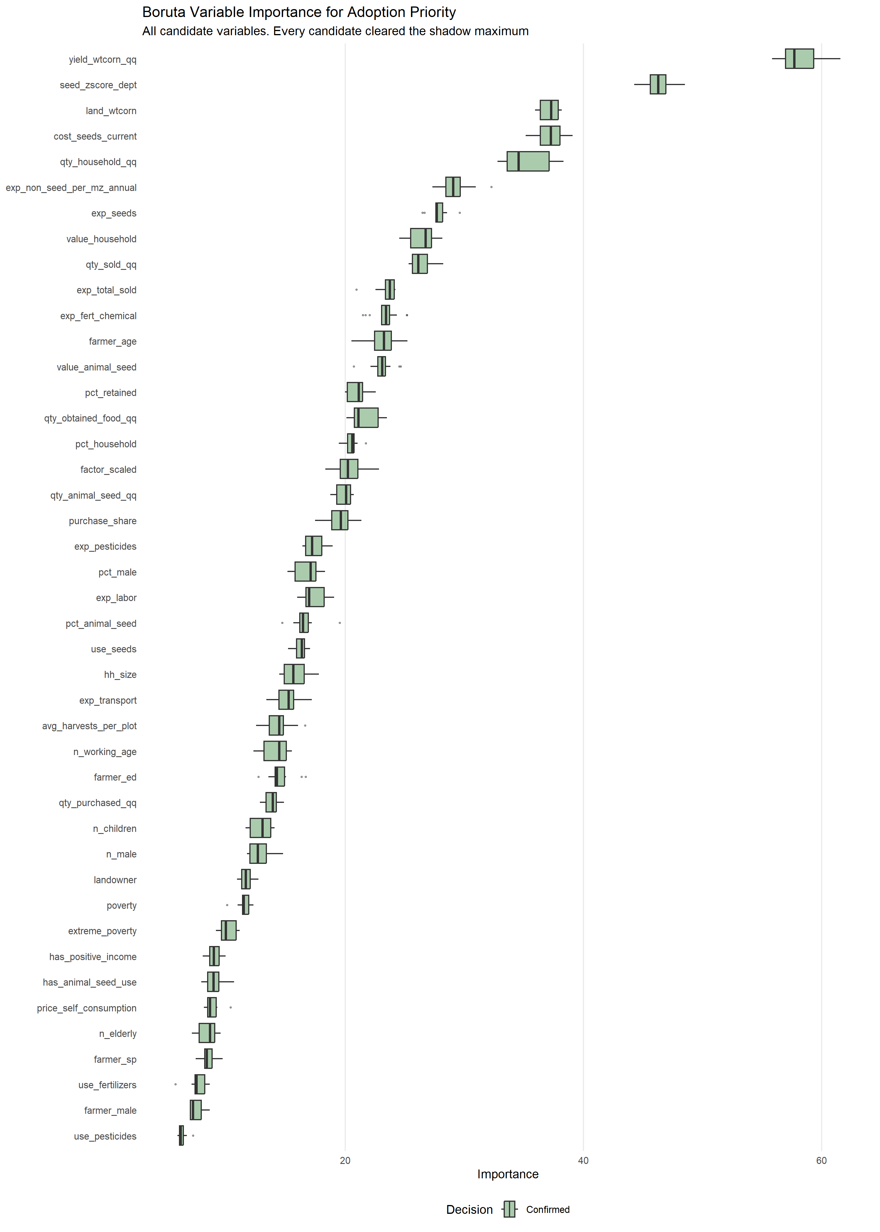
Boruta applies Random Forest importance to a model predicting adoption_priority from the candidate variables. At each iteration, each candidate is compared against a “shadow” version (its values randomly permuted across observations). A variable is Confirmed if its importance significantly exceeds the maximum shadow importance, Tentative if the evidence is inconclusive after maxRuns = 150 iterations, and Rejected if its importance falls below the shadow ceiling.

Horizontal boxplot chart of Boruta importance scores, one box per candidate variable on the y-axis, ordered by median importance, against importance on the x-axis. Boxes are colored by decision. Every candidate is confirmed, so the chart shows a single colour and no reference line: the whole set clears the shadow maximum, with the lowest median importance above 6. Importance spans roughly an order of magnitude between the weakest and the strongest predictor. — Figure 1: Boruta variable importance for adoption priority prediction

Table 4: Boruta Feature Selection Results

Boruta Feature Selection Results. Proxy outcome: adoption_priority (5-level ordinal). 43 confirmed, 0 tentative, 0 rejected
Variable	Decision	Median Imp.	Mean Imp.	Max Imp.
Boruta Feature Selection Results
Proxy outcome: adoption_priority (5-level ordinal). 43 confirmed, 0 tentative, 0 rejected
yield_wtcorn_qq	Confirmed	57.71	58.07	61.58
seed_zscore_dept	Confirmed	46.28	46.34	48.51
land_wtcorn	Confirmed	37.29	37.12	38.18
cost_seeds_current	Confirmed	37.27	37.23	39.08
qty_household_qq	Confirmed	34.56	35.26	38.33
exp_non_seed_per_mz_annual	Confirmed	29.07	29.19	32.27
exp_seeds	Confirmed	27.68	27.83	29.60
value_household	Confirmed	26.76	26.51	28.16
qty_sold_qq	Confirmed	26.12	26.37	28.22
exp_total_sold	Confirmed	23.75	23.46	24.21
exp_fert_chemical	Confirmed	23.43	23.37	25.18
farmer_age	Confirmed	23.25	23.02	25.22
value_animal_seed	Confirmed	23.11	23.07	24.65
pct_retained	Confirmed	21.13	21.08	22.55
qty_obtained_food_qq	Confirmed	21.11	21.65	23.48
pct_household	Confirmed	20.60	20.49	21.72
factor_scaled	Confirmed	20.21	20.33	22.82
qty_animal_seed_qq	Confirmed	20.07	19.85	20.71
purchase_share	Confirmed	19.62	19.59	21.34
exp_pesticides	Confirmed	17.21	17.45	18.95
pct_male	Confirmed	17.09	16.79	18.30
exp_labor	Confirmed	16.98	17.37	19.06
pct_animal_seed	Confirmed	16.45	16.63	19.53
use_seeds	Confirmed	16.35	16.17	17.04
hh_size	Confirmed	15.63	15.86	17.77
exp_transport	Confirmed	15.25	15.18	17.19
avg_harvests_per_plot	Confirmed	14.47	14.34	16.63
n_working_age	Confirmed	14.45	14.14	15.52
farmer_ed	Confirmed	14.26	14.56	16.67
qty_purchased_qq	Confirmed	13.93	13.82	14.86
n_children	Confirmed	13.06	12.96	14.07
n_male	Confirmed	12.67	12.81	14.77
landowner	Confirmed	11.64	11.75	12.70
poverty	Confirmed	11.48	11.49	12.28
extreme_poverty	Confirmed	9.96	10.15	11.14
has_positive_income	Confirmed	8.96	9.03	9.95
has_animal_seed_use	Confirmed	8.95	8.96	10.65
price_self_consumption	Confirmed	8.65	8.78	10.37
n_elderly	Confirmed	8.63	8.47	9.54
farmer_sp	Confirmed	8.38	8.43	9.70
use_fertilizers	Confirmed	7.50	7.67	8.63
farmer_male	Confirmed	7.21	7.46	8.62
use_pesticides	Confirmed	6.18	6.31	7.22
Boruta algorithm with maxRuns = 150, ranger importance source. Importance compared against shadow (permuted) variables.

Confirmed Variables Inform the Scoring Architecture

Boruta confirms all 43 candidates, with none tentative and none rejected. The step therefore does not discard variables here; what it provides is the importance ordering, which spans roughly an order of magnitude between the weakest confirmed predictor and the strongest. The scoring components — segment, economic benefit, improvement potential, scale, age, and the risk-aversion drivers — are built on that ordering, and each subsequent sweep operates on a parametric family of heuristics over these predictors.

Correlation Direction

The direction of association of each top-importance variable with the adoption priority proxy determines whether the scoring component should map “higher values → higher priority” or the inverse. Variables with Spearman correlation magnitude below 0.10 do not contribute usable directional signal and are flagged for review.

Table 5: Correlation of Top Variables with Adoption Priority

Variable Correlation with Adoption Priority. Spearman correlation (variables with Boruta importance ≥ 10)
Variable	ρ (Spearman)	Boruta Imp.	Direction
Variable Correlation with Adoption Priority
Spearman correlation (variables with Boruta importance ≥ 10)
yield_wtcorn_qq	−0.09	57.71	Weak/None
seed_zscore_dept	−0.46	46.28	Negative (↑ = lower priority)
land_wtcorn	0.22	37.29	Positive (↑ = higher priority)
cost_seeds_current	−0.21	37.27	Negative (↑ = lower priority)
qty_household_qq	0.22	34.56	Positive (↑ = higher priority)
exp_non_seed_per_mz_annual	−0.26	29.07	Negative (↑ = lower priority)
exp_seeds	−0.34	27.68	Negative (↑ = lower priority)
value_household	−0.02	26.76	Weak/None
qty_sold_qq	−0.05	26.12	Weak/None
exp_total_sold	−0.10	23.75	Negative (↑ = lower priority)
exp_fert_chemical	−0.09	23.43	Weak/None
farmer_age	0.00	23.25	Weak/None
value_animal_seed	0.00	23.11	Weak/None
pct_retained	0.13	21.13	Positive (↑ = higher priority)
qty_obtained_food_qq	0.00	21.11	Weak/None
pct_household	0.13	20.60	Positive (↑ = higher priority)
factor_scaled	0.03	20.21	Weak/None
qty_animal_seed_qq	0.08	20.07	Weak/None
purchase_share	−0.02	19.62	Weak/None
exp_pesticides	−0.12	17.21	Negative (↑ = lower priority)
pct_male	−0.01	17.09	Weak/None
exp_labor	−0.11	16.98	Negative (↑ = lower priority)
pct_animal_seed	0.05	16.45	Weak/None
use_seeds	−0.24	16.35	Negative (↑ = lower priority)
hh_size	0.08	15.63	Weak/None
exp_transport	−0.07	15.25	Weak/None
avg_harvests_per_plot	−0.01	14.47	Weak/None
n_working_age	0.05	14.45	Weak/None
farmer_ed	−0.06	14.26	Weak/None
qty_purchased_qq	0.00	13.93	Weak/None
n_children	0.08	13.06	Weak/None
n_male	0.07	12.67	Weak/None
landowner	−0.05	11.64	Weak/None
poverty	0.12	11.48	Positive (↑ = higher priority)
Positive: higher values → higher adoption priority. Negative: higher values → lower priority.

Phase D: Calibration Anchors

The Likely Adopters model is calibrated against a structured anchor set rather than fit to an outcome variable: the model parameters are tuned to reproduce, as closely as possible, the empirical adoption composition observed under the Semilla Nueva programme at multiple production coverage levels. The calibration anchors are of two kinds.

Empirical anchors (Semilla Nueva market composition). The Semilla Nueva market composition matrix reports the per-segment share of purchasing farmers at four production coverage levels: 5%, 10%, 20%, and 30%. The values at 5% and 10% correspond to the directly observed production coverage range of the 2022–2025 commercial period; the values at 20% and 30% are extrapolated from the same observational base using Gompertz sigmoid fits per segment. The revised matrix used here satisfies two structural requirements: per-segment cohort size is monotonically non-decreasing across production coverage levels, and no per-segment cohort size at any intermediate production coverage exceeds the corresponding population total at full production coverage.

A complementary land-size trajectory reports the average land planted in biofortified maize among purchasing farmers at the same four production coverage levels, interpreted as a P5–P95 trimmed-mean property of the adopting cohort, consistent with the trimming convention applied throughout the framework. Source values are reported in hectares and converted to manzanas using the conversion 1 ha = 1.4308 mz.

Calibration anchor set. The table below collates the five anchors used throughout this script: four empirical points from Semilla Nueva (Empirical) plus the structural anchor at full production coverage (Structural).

Anchor type	p	w_p	% OPV	% Low	% Mid	% High	Land overall (ha)	Land overall (mz)
Empirical (Semilla Nueva)	5%	1.0	17.8	59.6	12.6	10.0	0.44	0.6296
Empirical (Semilla Nueva)	10%	1.0	22.6	32.0	20.0	25.4	0.35	0.5008
Empirical (Semilla Nueva)	20%	1.0	41.6	17.0	15.7	25.7	0.53	0.7583
Empirical (Semilla Nueva)	30%	1.0	56.4	12.0	12.5	19.1	0.92	1.3163
Structural (population)	100%	0.5	—	—	—	—	—	—

The empirical row composition values are per-segment shares (%) of the purchasing-farmer cohort at each production coverage level (source: Semilla Nueva ex-ante segment composition estimate, April 2026). The land columns report the overall trimmed-mean land per farmer in the adopting cohort. The structural row at p = 100% is recovered from the segmented dataset itself: per-segment shares equal the population composition under survey-calibrated weights, and the land value equals the P5–P95 weighted trimmed mean of land_wtcorn across the universe.

Structural anchor (population at full production coverage). The composition at full production coverage equals the population composition by definition: at p = 1.0 every farmer in the segmented dataset has fully converted to biofortified maize. This anchor is recovered directly from the calibrated dataset using survey-calibrated weights and provides a natural asymptotic constraint that anchors the trajectory beyond the empirical range of Semilla Nueva observations.

A-priori weights. The four empirical anchors carry the direct empirical signal about adoption dynamics under the biofortification programme and are weighted equally with w_emp = 1.0. The population anchor at p = 1.0 represents the asymptotic composition of the universe; it is weighted at half the empirical anchors with w_str = 0.5, reflecting its auxiliary role.

Calibration distance. The MAD evaluation operates on relative deviations: each cell at each anchor contributes the absolute model-anchor error divided by the anchor value plus a small offset, so that all anchor cells contribute proportionally regardless of their absolute magnitude. Three composite distances are reported in every sweep: MAD farmers aggregates the deviations across per-segment cohort counts, MAD land aggregates the deviations across the overall land trajectory, and MAD global combines both on a common dimensionless basis. All sweeps in Phases E–G rank configurations on MAD global ascending: lower values indicate closer agreement with the anchor set.

Formal definition. Let \(\mathcal{S} = \{\text{OPV}, \text{Low}, \text{Mid}, \text{High}\}\) denote the segment set (\(|\mathcal{S}| = 4\)) and \(\mathcal{P} = \{0.05, 0.10, 0.20, 0.30, 1.00\}\) the anchor production coverage grid. The two component distances and the global distance are defined as

\[ \text{MAD}_{\text{farmers}} \;=\; \sum_{p \in \mathcal{P}} w_p \sum_{s \in \mathcal{S}} \frac{\bigl| N^{\text{model}}_{s,p} - N^{\text{anchor}}_{s,p} \bigr|} {N^{\text{anchor}}_{s,p} + \varepsilon_{\text{count}}} \]

\[ \text{MAD}_{\text{land}} \;=\; \sum_{p \in \mathcal{P}} w_p \frac{\bigl| \bar{L}^{\text{bio,model}}(p) - \bar{L}^{\text{bio,anchor}}(p) \bigr|} {\bar{L}^{\text{bio,anchor}}(p) + \varepsilon_{\text{land}}} \]

\[ \text{MAD}_{\text{global}} \;=\; \frac{\text{MAD}_{\text{farmers}}}{|\mathcal{S}|} \;+\; \text{MAD}_{\text{land}} \]

where \(w_p\) are the a-priori anchor weights (\(w_p = 1.0\) for the four empirical anchors, \(w_p = 0.5\) for the structural anchor at \(p = 1.0\)), \(\varepsilon_{\text{count}} = 1\) and \(\varepsilon_{\text{land}} = 0.01\) are the small offsets that prevent division-by-zero on cohort cells that are vanishingly small at low production coverage, and \(|\mathcal{S}| = 4\) normalises the farmer component to a per-segment scale before composing with the land component on a common dimensionless basis.

The implementation aligns the modelled trajectory grid and the anchor grid through an explicit integer key (production coverage multiplied by 1000 and rounded), eliminating dependence on floating-point equality between the two grids.

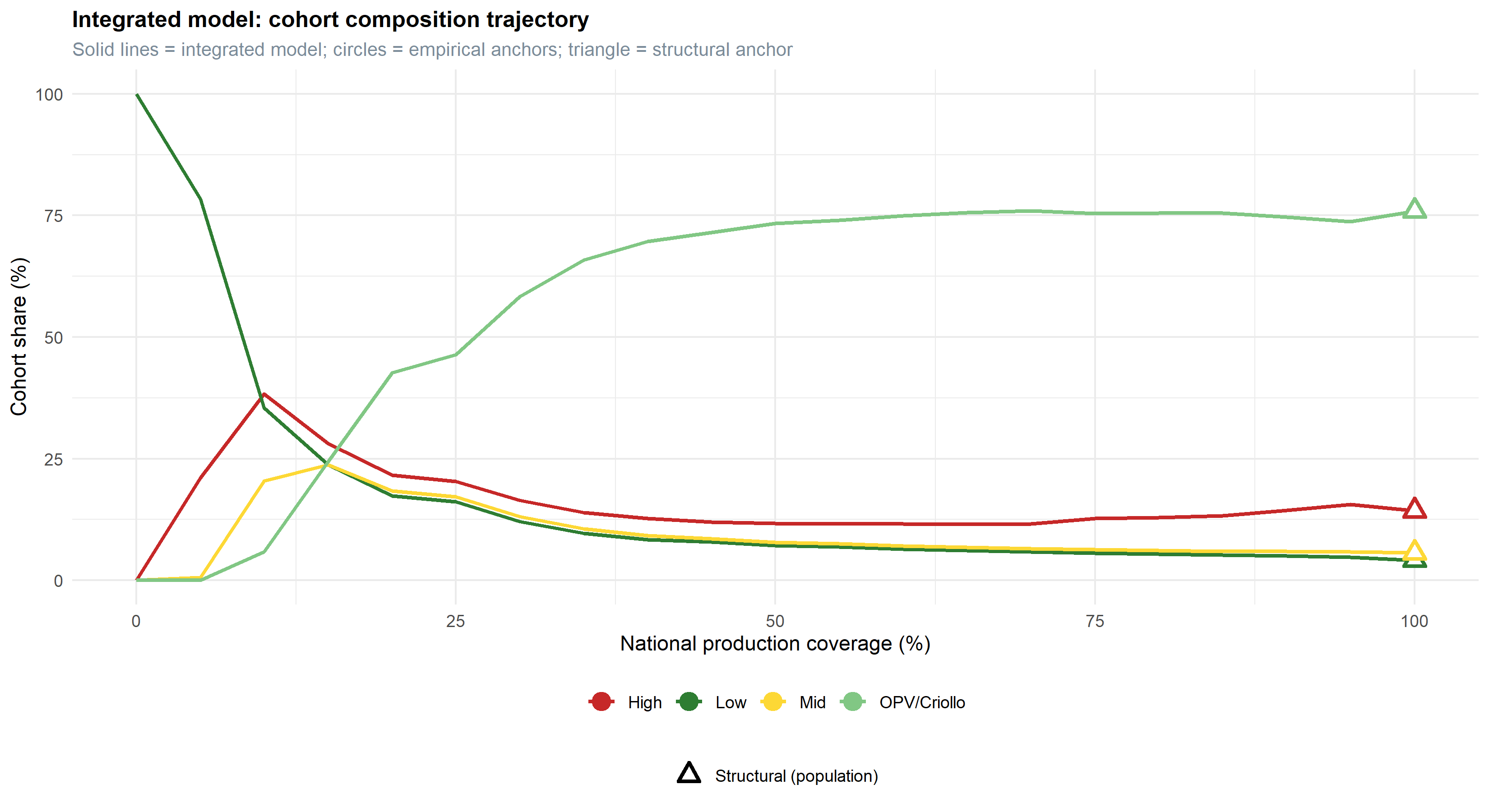
The five-anchor set is held fixed across every sweep in this script; what changes is the model configuration whose calibration distance is evaluated against it. The visualisation of the integrated model trajectory against these anchors appears in Phase H3.

Phase E: Scoring Sensitivity Sweeps

The scoring engine assigns each farmer a composite score from five components: a categorical segment score over the four segments (Low, OPV/Criollo, Mid, High); a continuous economic-benefit score over projected income increment; a continuous improvement-potential score over current per-area input expenditure (inverse direction: lower expenditure indicates higher potential for productivity gains); a continuous scale score over land area planted in white maize; and a continuous age score over the head-of-household age (inverse direction: younger heads of household show higher technological openness). Each continuous score is a step function over percentile breakpoints of the underlying variable, yielding integer levels that align cardinality across components.

Phase E explores the architectural choices of the scoring engine through four sequential sweeps. Each sweep inherits the best configuration from the previous one, so the search proceeds along a one-dimensional path rather than a full grid: the heuristic configuration (E2) is selected on individual-component sensitivity, the segment scheme (E3) is selected against the heuristic configuration, and the weight vector (E4) is selected against the heuristic and segment configurations.

E2 — Sensitivity to Scoring Heuristics

Each of the four non-segment scoring components is varied independently while the others are held at reference defaults. The univariate best variant of each component is selected on minimum global MAD.

E2.1 — score_economic Breakpoints

The economic-benefit score uses three percentile breakpoints over income_increment to assign farmers to four bands (with an additional fifth band for non-positive increments). Three variants of the breakpoint vector are evaluated.

Table 6: Sensitivity to score_economic Breakpoints

Sensitivity to score_economic breakpoints. Other components held at reference defaults; ordered by global MAD
Component	Variant	Label	MAD farmers	MAD land (mz)	MAD global
Sensitivity to score_economic breakpoints
Other components held at reference defaults; ordered by global MAD
score_economic	econ_soft	Soft (P20/P40/P60)	13.068	28.157	31.424
score_economic	econ_default	Default (P25/P50/P75)	13.476	32.711	36.080
score_economic	econ_demanding	Demanding (P50/P70/P90)	14.261	55.305	58.870

E2.2 — score_improvement Breakpoints

The improvement-potential score uses four percentile breakpoints over exp_total_per_mz_annual (inverse direction). Three variants of the breakpoint vector are evaluated.

Table 7: Sensitivity to score_improvement Breakpoints

Sensitivity to score_improvement breakpoints. Other components held at reference defaults; ordered by global MAD
Component	Variant	Label	MAD farmers	MAD land (mz)	MAD global
Sensitivity to score_improvement breakpoints
Other components held at reference defaults; ordered by global MAD
score_improvement	impr_soft	Soft (P30/P60/P80/P95)	13.265	26.526	29.843
score_improvement	impr_default	Default (P25/P50/P75/P90)	13.476	32.711	36.080
score_improvement	impr_demanding	Demanding (P10/P25/P50/P75)	13.502	46.048	49.424

E2.3 — score_scale Breakpoints

The scale score uses four percentile breakpoints over land_wtcorn to discriminate among farmer scales. Three variants of the breakpoint vector are evaluated.

Table 8: Sensitivity to score_scale Breakpoints

Sensitivity to score_scale breakpoints. Other components held at reference defaults; ordered by global MAD
Component	Variant	Label	MAD farmers	MAD land (mz)	MAD global
Sensitivity to score_scale breakpoints
Other components held at reference defaults; ordered by global MAD
score_scale	scale_default	Default (P25/P50/P75)	13.476	32.711	36.080
score_scale	scale_soft	Soft (P33/P66/P90)	13.661	40.889	44.304
score_scale	scale_demanding	Demanding (P50/P75/P90)	13.775	43.178	46.622

E2.4 — score_age Breakpoints

The age score uses cutoffs over head-of-household age (inverse direction: younger ages map to higher scores). Three variants are evaluated.

Table 9: Sensitivity to score_age Breakpoints

Sensitivity to score_age breakpoints. Other components held at reference defaults; ordered by global MAD
Component	Variant	Label	MAD farmers	MAD land (mz)	MAD global
Sensitivity to score_age breakpoints
Other components held at reference defaults; ordered by global MAD
score_age	age_55_w10_neutral_edges	Peak 55 ±10 \| neutral_edges	13.260	29.370	32.685
score_age	age_55_w10_decreasing	Peak 55 ±10 \| decreasing	13.286	29.900	33.222
score_age	age_50_w5_elder_priority	Peak 50 ±5 \| elder_priority	13.049	30.546	33.808
score_age	age_50_w5_neutral_edges	Peak 50 ±5 \| neutral_edges	13.034	30.949	34.207
score_age	age_50_w5_decreasing	Peak 50 ±5 \| decreasing	13.073	31.571	34.839
score_age	age_45_w10_decreasing	Peak 45 ±10 \| decreasing	12.926	32.258	35.490
score_age	age_55_w5_elder_priority	Peak 55 ±5 \| elder_priority	13.413	32.382	35.735
score_age	age_50_w10_decreasing	Peak 50 ±10 \| decreasing	13.383	32.427	35.773
score_age	age_55_w5_decreasing	Peak 55 ±5 \| decreasing	13.476	32.711	36.080
score_age	age_45_w5_decreasing	Peak 45 ±5 \| decreasing	13.004	33.045	36.296
score_age	age_55_w5_young_priority	Peak 55 ±5 \| young_priority	13.480	33.900	37.270
score_age	age_45_w5_young_priority	Peak 45 ±5 \| young_priority	13.018	34.567	37.821

E2.5 — Best Heuristic per Component

The best heuristic per component is selected on minimum global MAD within each individual sweep. The combined configuration is carried forward as the reference scoring heuristic for the subsequent sweeps in this phase.

Table 10: Selected Heuristic Configuration (Univariate Best per Component)

Selected heuristic configuration (univariate best per component). Variants minimising global MAD within each component sweep
Component	Variant	Label	MAD farmers	MAD land (mz)	MAD global
Selected heuristic configuration (univariate best per component)
Variants minimising global MAD within each component sweep
score_economic	econ_soft	Soft (P20/P40/P60)	13.068	28.157	31.424
score_improvement	impr_soft	Soft (P30/P60/P80/P95)	13.265	26.526	29.843
score_scale	scale_default	Default (P25/P50/P75)	13.476	32.711	36.080
score_age	age_55_w10_neutral_edges	Peak 55 ±10 \| neutral_edges	13.260	29.370	32.685

E3 — Sensitivity to Segment-Priority Schemes

The segment-priority sweep explores two families of cardinal configurations. A steep family (gap of 20 or more points between consecutive segments) tests whether the segment component, treated as the dominant input to the composite score, reproduces the empirical anchor pattern on its own. A compressed family (gap of 5 to 15 points between consecutive segments) tests an alternative architecture in which the segment component provides a weak categorical prior and the discrimination among farmers is carried by the economic, improvement, scale, age, and risk-aversion components.

The heuristic configuration from E2.5 is held fixed during this sweep.

Table 11: Sensitivity to Segment-Priority Schemes

Sensitivity to segment-priority schemes. Best heuristics from E2 fixed; component weights at reference; ordered by global MAD
Scheme	Low	OPV	Mid	High	MAD farmers	MAD land (mz)	MAD global
Sensitivity to segment-priority schemes
Best heuristics from E2 fixed; component weights at reference; ordered by global MAD
lhm_shallow	100	45	70	85	11.166	10.026	12.818
lmh_steep	100	20	75	50	10.673	11.327	13.995
lhm_steep	100	50	60	65	11.639	11.469	14.378
lmo_balanced	100	50	75	20	11.817	13.560	16.514
lmh_shallow	100	40	85	70	11.286	17.456	20.278
lom_default	100	80	40	10	12.783	22.528	25.723
flat_low_opv	70	60	50	45	12.536	26.872	30.007
flat_lo_demote	80	70	55	40	12.536	26.872	30.007
fully_flat	60	55	50	45	12.670	29.329	32.497
low_opv_paired	75	70	50	30	12.712	29.526	32.704
flat_lhm	65	50	55	60	13.210	29.654	32.956

E4 — Sensitivity to Component Weights

The component weights are the relative contributions of the five scoring components to the composite score. Holding the heuristic configuration from E2 and the segment scheme from E3 fixed, the weight vector is varied across plausible neighbourhoods of the reference baseline.

The grid is constructed by varying the segment weight on a coarse range. The age and scale weights are held at their reference values (0.07 and 0.08), so the perturbation operates primarily on the segment / economic / improvement balance. The segment weight is bounded at 0.60 from above: a segment weight above this threshold produces a ranking in which the categorical segment classification dominates the composite to the point where intra-segment variation in the other components becomes irrelevant.

Table 12: Sensitivity to Component Weights

Sensitivity to component weights. Best heuristics from E2 and best segment scheme from E3 fixed; ordered by global MAD
w_seg	w_econ	w_impr	w_scale	w_age	MAD farmers	MAD land (mz)	MAD global
Sensitivity to component weights
Best heuristics from E2 and best segment scheme from E3 fixed; ordered by global MAD
0.600	0.162	0.088	0.080	0.070	8.507	3.825	5.951
0.600	0.200	0.050	0.080	0.070	8.474	3.864	5.982
0.600	0.125	0.125	0.080	0.070	8.943	4.089	6.324
0.500	0.280	0.070	0.080	0.070	9.713	6.271	8.699
0.500	0.227	0.123	0.080	0.070	10.080	6.676	9.196
0.500	0.175	0.175	0.080	0.070	10.398	7.063	9.662
0.400	0.360	0.090	0.080	0.070	10.770	8.840	11.533
0.400	0.293	0.157	0.080	0.070	11.304	10.632	13.458
0.400	0.225	0.225	0.080	0.070	11.801	13.756	16.707

Recommended Scoring Configuration

The recommended scoring configuration combines the best heuristics from E2, the best segment scheme from E3, and the best component-weight vector from E4. This configuration is carried forward to Phase F as the base scoring on which the risk-aversion penalty is applied.

Phase F: Risk-Aversion Sweep

The risk-aversion penalty discounts the composite score of each farmer by an explicit measure of vulnerability to crop loss. Three risk drivers are combined into the penalty: a yield-variability driver (the per-farmer variability of expected yield against the departmental reference), a cost-to-output ratio driver (the per-farmer ratio of input expenditure to projected gross production value), and a land-scale driver (the per-farmer land area in white maize, with smaller plots interpreted as carrying greater relative risk from a single-season loss). A fourth structural driver, the projected-loss driver, captures the disincentive associated with a projected negative income increment and is held fixed by design at α_loss = 1.0 across all configurations: this reflects its structural role as a deterministic disincentive rather than a calibrated component.

The penalty is shaped by a logistic function with slope β over the weighted aggregate of the three calibrated drivers, and is subtracted from the composite score with weight w_R. Two variants of the driver formulation are evaluated in parallel: the Z variant standardises each driver against its departmental mean and standard deviation (yielding interpretable z-scores), while the A variant normalises each driver against its population P1–P99 range. Both variants are explored under a five-dimensional joint sweep over α_yield, α_ratio, α_land, β, and w_R, ranked on the same MAD distance used in Phase E.

Table 13: Top 5 Risk-Aversion Configurations per Driver Variant

Top 5 risk-aversion configurations per variant. Z = departmental z-scores; A = absolute values normalised via P1–P99
α_yield	α_ratio	α_land	β	w_R	MAD farmers	MAD land (mz)	MAD global
Top 5 risk-aversion configurations per variant
Z = departmental z-scores; A = absolute values normalised via P1–P99
a
0.20	0.10	0.70	2.00	0.40	5.873	1.601	3.069
0.20	0.30	0.50	2.50	0.40	5.569	1.680	3.072
0.00	0.00	1.00	2.50	0.30	6.795	1.387	3.086
0.10	0.00	0.90	2.50	0.30	6.232	1.529	3.087
0.30	0.10	0.60	2.50	0.40	5.854	1.631	3.094
z
0.00	0.10	0.90	1.00	0.40	5.618	1.506	2.910
0.00	0.00	1.00	1.00	0.40	6.169	1.400	2.943
0.00	0.00	1.00	1.50	0.30	5.769	1.518	2.961
0.00	0.20	0.80	1.00	0.40	5.322	1.651	2.981
0.00	0.30	0.70	1.00	0.40	4.983	1.752	2.998

Combined Configuration Carried Forward

The best risk-aversion configuration is combined with the best scoring configuration from Phase E. This combined scoring + risk model is the entry point for the continuous-adoption sweeps in Phase G.

Phase G: Continuous Adoption Sweeps

The continuous adoption model assigns each farmer to one of three behavioural profiles based on white-maize land area: small (S) with near-binary adoption (rapid full conversion once the farmer enters the ranking), medium (M) with sigmoid adoption (gradual conversion shaped by a logistic curve), and large (L) with gradual adoption (slow accumulation that approaches saturation only at high national production coverage). The per-farmer conversion ratio r_i(p) depends on the farmer’s profile and on the farmer’s entry point p_entry in the global ranking.

The sweep explores three design axes sequentially, with each axis inheriting the best configuration from the previous one:

G2 — Floor values define the minimum conversion ratio achieved immediately upon entry into the ranking, per profile.
G3 — Steepness coefficients define the slope of the conversion curve between entry and saturation, per profile.
G4 — Profile cutoffs define the land-area boundaries that assign farmers to profiles S, M, or L.

Phase G inherits the combined scoring + risk configuration from Phase F.

G2 — Floor Values per Profile

The floor value of each profile is the conversion ratio achieved immediately upon entry into the ranking. A high floor models a near-step adoption (“once the farmer decides, all land is committed”); a low floor models a gradual scaling that begins from a small fraction of the land. The grid varies all three floors independently across plausible ranges.

Table 14: Sensitivity to Floor Values per Profile

Sensitivity to floor values per profile. Steepness coefficients and cutoffs held at reference; ordered by global MAD
floor_S	floor_M	floor_L	MAD farmers	MAD land (mz)	MAD global
Sensitivity to floor values per profile
Steepness coefficients and cutoffs held at reference; ordered by global MAD
0.95	0.50	0.20	5.172	1.119	2.412
0.95	0.50	0.10	5.246	1.226	2.538
0.95	0.50	0.05	5.283	1.302	2.623
0.85	0.50	0.20	5.669	1.246	2.664
0.95	0.50	0.02	5.305	1.367	2.694
0.95	0.40	0.20	5.485	1.387	2.758
0.85	0.50	0.10	5.743	1.353	2.789
0.95	0.40	0.10	5.560	1.482	2.872
0.85	0.50	0.05	5.781	1.429	2.874
0.85	0.50	0.02	5.803	1.494	2.945
0.95	0.40	0.05	5.597	1.549	2.949
0.85	0.40	0.20	5.983	1.514	3.009
0.95	0.40	0.02	5.619	1.606	3.011
0.85	0.40	0.10	6.057	1.608	3.123
0.85	0.40	0.05	6.094	1.676	3.200
0.85	0.40	0.02	6.117	1.729	3.258

G3 — Steepness Coefficients per Profile

The steepness coefficient k governs the curvature of the conversion ratio between entry and saturation: large k produces a near-step curve (rapid jump from floor to ceiling), small k produces a gradual sigmoid (smooth scaling over an extended production coverage range). Holding the best floor values from G2 and the reference cutoff scheme, the steepness coefficients are explored independently across the three profiles.

Table 15: Sensitivity to Steepness Coefficients per Profile

Sensitivity to steepness coefficients per profile. Best floors from G2 fixed; cutoffs at reference; ordered by global MAD
k_S	k_M	k_L	MAD farmers	MAD land (mz)	MAD global
Sensitivity to steepness coefficients per profile
Best floors from G2 fixed; cutoffs at reference; ordered by global MAD
8.00	4.00	0.50	5.041	1.062	2.322
8.00	4.00	1.00	5.042	1.063	2.323
12.00	4.00	0.50	5.050	1.062	2.325
8.00	4.00	1.50	5.044	1.064	2.326
16.00	4.00	0.50	5.054	1.063	2.326
12.00	4.00	1.00	5.051	1.063	2.326
16.00	4.00	1.00	5.055	1.064	2.327
12.00	4.00	1.50	5.053	1.065	2.329
8.00	4.00	2.00	5.047	1.067	2.329
16.00	4.00	1.50	5.057	1.066	2.330
12.00	4.00	2.00	5.056	1.068	2.332
16.00	4.00	2.00	5.060	1.068	2.333
8.00	8.00	0.50	5.139	1.098	2.383
8.00	8.00	1.00	5.140	1.099	2.384
8.00	8.00	1.50	5.143	1.099	2.385
12.00	8.00	0.50	5.148	1.099	2.386
16.00	8.00	0.50	5.152	1.099	2.387
12.00	8.00	1.00	5.149	1.100	2.387
12.00	8.00	1.50	5.152	1.100	2.388
8.00	8.00	2.00	5.146	1.102	2.388
16.00	8.00	1.00	5.153	1.100	2.388
16.00	8.00	1.50	5.155	1.100	2.389
12.00	8.00	2.00	5.155	1.103	2.391
16.00	8.00	2.00	5.158	1.103	2.392

G4 — Profile Cutoff Sensitivity

The profile cutoffs S/M and M/L define the land-area boundaries that assign farmers to profiles S, M, or L. Holding the best floors from G2 and the best steepness coefficients from G3, the cutoff grid explores plausible refinements of the empirical land percentiles used as reference.

Table 16: Sensitivity to Profile Cutoffs

Sensitivity to profile cutoffs. Best floors from G2 and best steepness from G3 fixed; ordered by global MAD
cut S/M (mz)	cut M/L (mz)	MAD farmers	MAD land (mz)	MAD global
Sensitivity to profile cutoffs
Best floors from G2 and best steepness from G3 fixed; ordered by global MAD
1.25	3.00	4.518	0.997	2.126
1.50	3.00	4.489	1.013	2.135
1.00	7.00	4.803	0.952	2.153
1.00	6.00	4.806	0.955	2.156
1.00	5.00	4.819	0.965	2.170
1.25	4.00	4.494	1.048	2.171
1.50	4.00	4.477	1.060	2.179
1.25	5.00	4.487	1.069	2.190
1.00	4.00	4.848	0.983	2.195
1.50	5.00	4.480	1.080	2.200
1.25	6.00	4.491	1.084	2.207
1.25	7.00	4.492	1.087	2.209
1.50	6.00	4.484	1.096	2.217
1.50	7.00	4.485	1.098	2.220
1.00	3.00	4.890	1.007	2.230

Phase H: Integrated Model Evaluation

The integrated model combines all best configurations from Phases E, F, and G: the heuristic configuration from E2, the segment scheme from E3, the component weights from E4, the risk-aversion variant and coefficients from F, and the continuous-adoption parameters (floors, steepness, cutoffs) from G. The integrated model is evaluated against the five-anchor calibration set and exported as the final model artefact consumed when applying the model.

Integrated Model Calibration Summary

Table 17: Integrated Model — Calibration Distance Against Anchor Set

Integrated model — calibration distance. Relative mean absolute deviation against the five calibration anchors
Model	MAD farmers	MAD land (mz)	MAD global
Integrated model — calibration distance
Relative mean absolute deviation against the five calibration anchors
Integrated (scoring + risk + continuous adoption)	4.518	0.997	2.126

Trajectory Visualization Against Anchors

The integrated model’s trajectory is visualised against the five calibration anchors: four empirical points from the Semilla Nueva market composition matrix (circles) and one structural point recovered from the population at full production coverage (triangle). The four segment trajectories appear as solid lines on a percentage-share basis.

Line chart with national production coverage (percent) on the x-axis and cohort share (percent) on the y-axis. Four solid lines, one per farmer segment, trace the integrated model's composition trajectory as coverage grows. Overlaid markers show the calibration anchors: circles for the four empirical Semilla Nueva points and a triangle for the structural point at full coverage. The model lines pass close to their corresponding anchor markers, showing the calibrated fit. — Figure 2: Integrated model trajectory against the calibration anchors

Final Configuration Summary

The full set of parameters constituting the determined Likely Adopters model is reported below. This configuration is exported as a single artefact in the model registry and read back when applying the model.

Table 18: Determined Likely Adopters Model Configuration

Determined Likely Adopters model configuration. Calibrated against five anchors on the baseline configuration (2022 seed, current subsidy)
Component	Setting
Determined Likely Adopters model configuration
Calibrated against five anchors on the baseline configuration (2022 seed, current subsidy)
Segment scheme	lhm_shallow: Low=100, OPV=45, Mid=70, High=85
Component weights	seg=0.6, econ=0.162, impr=0.088, scale=0.08, age=0.07
Heuristic — score_economic	Soft (P20/P40/P60)
Heuristic — score_improvement	Soft (P30/P60/P80/P95)
Heuristic — score_scale	Default (P25/P50/P75)
Heuristic — score_age	Peak 55 ±10 \| neutral_edges
Risk variant	z
Risk drivers (α_yield, α_ratio, α_land)	yield=0, ratio=0.1, land=0.9
Risk structural loss coefficient (α_loss)	1.00
Risk slope (β)	1.00
Risk weight (w_R)	0.40
Profile cutoffs (S/M, M/L)	S/M=1.25 mz, M/L=3 mz
Profile floors (S, M, L)	floor_S=0.95, floor_M=0.5, floor_L=0.2
Profile steepness (k_S, k_M, k_L)	k_S=8, k_M=4, k_L=0.5
Entry-size cutoffs (S/M, M/L)	S/M=1.5 mz, M/L=7 mz
Entry-size coefficients (S, M, L)	coef_S=0.95, coef_M=0.5, coef_L=0.2
MAD farmers (integrated)	4.518
MAD land (mz, integrated)	0.997
MAD global (integrated)	2.126

Summary

Determination Pipeline

The Likely Adopters model is determined through a sequential, anchor-driven calibration: variable selection (Phase B–C) identifies the predictors with statistically significant association with the adoption priority proxy, the calibration anchor set (Phase D) defines the target against which all subsequent configurations are evaluated, the scoring sensitivity sweeps (Phase E) select the heuristic configuration, segment scheme, and component weights, the risk-aversion sweep (Phase F) selects the driver variant and the coefficients of the risk penalty, and the continuous-adoption sweeps (Phase G) select the floor values, steepness coefficients, and profile cutoffs of the per-farmer conversion curve.

Single Calibration, Universal Application

The determination is performed once on the baseline configuration (2022 seed × current subsidy). The structural parameters identified depend on the joint distribution of farmer characteristics, not on the magnitude of the projected economic benefit. The single calibration therefore produces the model configuration applicable across the seed by subsidy combinations evaluated by the downstream scoring engine.

Anchor-Based Calibration

The calibration targets are five anchor points derived from the Semilla Nueva market composition matrix (four empirical production coverage levels) plus one structural anchor (population composition at full production coverage). The MAD distance ranks every configuration on a common dimensionless basis, enabling sequential one-axis optimisation across the four phases. The integrated model trajectory reproduces the empirical anchors with low residual deviation, which is what the continuous-adoption projections downstream rest on.