| Farmer Population Scaling Factor | |
| Alignment of ENCOVI estimates with INE agricultural census | |
| Metric | Value |
|---|---|
| INE reference (2011) | 1,299,377 |
| ENCOVI weighted total | 664,971 |
| Scaling factor | 1.9540 |
| Source: INE (2011) — Distribución de hogares agropecuarios según tipología | |
MAGA Weight Calibration
Module 2: Economic Impact
Why Calibrate to MAGA?
Survey data and administrative records often produce different estimates of agricultural activity. ENCOVI 2023 captures detailed farmer-level information but uses a general population sampling frame that may under- or over-represent certain agricultural regions. MAGA (Ministerio de Agricultura, Ganadería y Alimentación) publishes official departmental statistics based on comprehensive agricultural monitoring.
By calibrating ENCOVI survey weights to match MAGA totals, we achieve:
- Administrative consistency — Weighted estimates align with official government statistics used in policy planning
- Improved representativeness — Correct for differential sampling rates across agricultural departments
- Credibility for stakeholders — Results match published figures that donors and policymakers reference
This calibration step is particularly important for economic impact projections, where departmental production volumes directly affect estimated benefits from biofortified maize adoption.
Calibration Approach
The calibration process adjusts individual survey weights so that weighted departmental totals for production (quintales) and cultivated land (manzanas) match MAGA 2023 official statistics.
Data Sources
| Source | Purpose |
|---|---|
| ENCOVI 2023 | Farmer-level characteristics, original survey weights |
| MAGA 2023 | Departmental targets for production and land area |
| INE 2011 | Total agricultural household reference (1,299,377) |
Calibration Variables
- Production (
total_production) — Total white maize harvested in quintales - Land (
land_wtcorn) — Cultivated white maize area in manzanas
Both variables are calibrated simultaneously within each department using linear calibration, ensuring weighted totals match MAGA targets exactly.
Initial Weight Scaling
Before departmental calibration, we apply a scaling factor to align ENCOVI’s total agricultural household estimate with official INE census figures.
NoteScaling Factor
At 1.954, the factor places ENCOVI’s original weights at around half the agricultural population the INE census estimates. ENCOVI draws on a general population sampling frame, not an agriculture-specific one, and the factor closes that gap before the departmental calibration runs.
Pre-Calibration Diagnostic
Before applying calibration, we compare ENCOVI weighted estimates against MAGA departmental targets to quantify the magnitude of discrepancies.
| Pre-Calibration: ENCOVI vs MAGA Comparison | ||||||||
| Weighted estimates before departmental calibration | ||||||||
| Department | N (sample) |
Production (qq)
|
Land (mz)
|
|||||
|---|---|---|---|---|---|---|---|---|
| ENCOVI | MAGA | Ratio | ENCOVI | MAGA | Ratio | |||
| Alta Verapaz | 99 | 12,521,541 | 5,296,634 | 2.36 | 338,833 | 252,979 | 1.34 | |
| Baja Verapaz | 47 | 7,294,761 | 720,542 | 10.12 | 124,530 | 40,233 | 3.10 | |
| Chimaltenango | 84 | 9,976,272 | 1,065,264 | 9.37 | 240,782 | 34,835 | 6.91 | |
| Chiquimula | 97 | 9,367,005 | 1,518,844 | 6.17 | 201,754 | 65,717 | 3.07 | |
| El Progreso | 28 | 1,129,470 | 367,087 | 3.08 | 37,795 | 20,283 | 1.86 | |
| Escuintla | 28 | 942,767 | 528,828 | 1.78 | 31,456 | 10,216 | 3.08 | |
| Guatemala | 14 | 2,937,732 | 816,778 | 3.60 | 71,871 | 28,939 | 2.48 | |
| Huehuetenango | 64 | 3,493,937 | 4,023,703 | 0.87 | 128,316 | 156,526 | 0.82 | |
| Izabal | 85 | 6,386,107 | 1,254,753 | 5.09 | 149,271 | 30,116 | 4.96 | |
| Jalapa | 54 | 3,851,500 | 1,095,143 | 3.52 | 77,082 | 40,300 | 1.91 | |
| Jutiapa | 116 | 5,869,034 | 2,646,775 | 2.22 | 152,504 | 86,098 | 1.77 | |
| Petén | 73 | 5,612,033 | 10,658,142 | 0.53 | 147,838 | 356,518 | 0.41 | |
| Quetzaltenango | 33 | 1,287,887 | 2,580,710 | 0.50 | 60,794 | 62,296 | 0.98 | |
| Quiché | 74 | 9,399,415 | 5,171,702 | 1.82 | 219,059 | 224,720 | 0.97 | |
| Retalhuleu | 22 | 2,924,853 | 1,129,300 | 2.59 | 72,074 | 29,346 | 2.46 | |
| Sacatepéquez | 22 | 363,951 | 321,895 | 1.13 | 25,534 | 12,495 | 2.04 | |
| San Marcos | 46 | 4,081,664 | 2,538,994 | 1.61 | 105,051 | 74,815 | 1.40 | |
| Santa Rosa | 70 | 1,757,133 | 886,464 | 1.98 | 88,869 | 23,071 | 3.85 | |
| Sololá | 21 | 749,294 | 810,483 | 0.92 | 23,154 | 24,550 | 0.94 | |
| Suchitepéquez | 27 | 2,545,635 | 555,180 | 4.59 | 73,293 | 11,689 | 6.27 | |
| Totonicapán | 40 | 721,686 | 999,141 | 0.72 | 36,995 | 42,234 | 0.88 | |
| Zacapa | 55 | 3,822,529 | 774,130 | 4.94 | 85,968 | 23,755 | 3.62 | |
| Total | — | 1,199 | 97,036,208 | 45,760,490 | — | 2,492,824 | 1,651,732 | — |
| Ratio = ENCOVI / MAGA. Values far from 1.0 indicate large discrepancies requiring calibration. Red highlight: ratio < 0.5 or > 2.0 |
||||||||
WarningSubstantial Discrepancies
Several departments show ratios far from 1.0, indicating that ENCOVI weighted estimates diverge substantially from MAGA administrative data. Calibration corrects these discrepancies departmentally.
Post-Calibration Validation
After applying departmental calibration, we verify that weighted totals match MAGA targets exactly.
| Post-Calibration Validation: ENCOVI vs MAGA | ||||||||
| Calibrated weighted estimates should match MAGA targets (ratio ≈ 1.00) | ||||||||
| Department | N (sample) |
Production (qq)
|
Land (mz)
|
|||||
|---|---|---|---|---|---|---|---|---|
| Calibrated | MAGA | Ratio | Calibrated | MAGA | Ratio | |||
| Alta Verapaz | 99 | 5,296,634 | 5,296,634 | 1.0000 | 252,979 | 252,979 | 1.0000 | |
| Baja Verapaz | 47 | 720,542 | 720,542 | 1.0000 | 40,233 | 40,233 | 1.0000 | |
| Chimaltenango | 84 | 1,065,264 | 1,065,264 | 1.0000 | 34,835 | 34,835 | 1.0000 | |
| Chiquimula | 97 | 1,518,844 | 1,518,844 | 1.0000 | 65,717 | 65,717 | 1.0000 | |
| El Progreso | 28 | 367,087 | 367,087 | 1.0000 | 20,283 | 20,283 | 1.0000 | |
| Escuintla | 28 | 528,828 | 528,828 | 1.0000 | 10,216 | 10,216 | 1.0000 | |
| Guatemala | 14 | 816,778 | 816,778 | 1.0000 | 28,939 | 28,939 | 1.0000 | |
| Huehuetenango | 64 | 4,023,703 | 4,023,703 | 1.0000 | 156,526 | 156,526 | 1.0000 | |
| Izabal | 85 | 1,254,753 | 1,254,753 | 1.0000 | 30,116 | 30,116 | 1.0000 | |
| Jalapa | 54 | 1,095,143 | 1,095,143 | 1.0000 | 40,300 | 40,300 | 1.0000 | |
| Jutiapa | 116 | 2,646,775 | 2,646,775 | 1.0000 | 86,098 | 86,098 | 1.0000 | |
| Petén | 73 | 10,658,142 | 10,658,142 | 1.0000 | 356,518 | 356,518 | 1.0000 | |
| Quetzaltenango | 33 | 2,580,710 | 2,580,710 | 1.0000 | 62,296 | 62,296 | 1.0000 | |
| Quiché | 74 | 5,171,702 | 5,171,702 | 1.0000 | 224,720 | 224,720 | 1.0000 | |
| Retalhuleu | 22 | 1,129,300 | 1,129,300 | 1.0000 | 29,346 | 29,346 | 1.0000 | |
| Sacatepéquez | 22 | 321,895 | 321,895 | 1.0000 | 12,495 | 12,495 | 1.0000 | |
| San Marcos | 46 | 2,538,994 | 2,538,994 | 1.0000 | 74,815 | 74,815 | 1.0000 | |
| Santa Rosa | 70 | 886,464 | 886,464 | 1.0000 | 23,071 | 23,071 | 1.0000 | |
| Sololá | 21 | 810,483 | 810,483 | 1.0000 | 24,550 | 24,550 | 1.0000 | |
| Suchitepéquez | 27 | 555,180 | 555,180 | 1.0000 | 11,689 | 11,689 | 1.0000 | |
| Totonicapán | 40 | 999,141 | 999,141 | 1.0000 | 42,234 | 42,234 | 1.0000 | |
| Zacapa | 55 | 774,130 | 774,130 | 1.0000 | 23,755 | 23,755 | 1.0000 | |
| Total | — | 1,199 | 45,760,490 | 45,760,490 | — | 1,651,732 | 1,651,732 | — |
| Ratio = Calibrated / MAGA. Values of 1.0000 confirm exact calibration. Green highlight: both ratios within ±0.1% of target. |
||||||||
NoteCalibration Result
The 22 departments reach a ratio of 1.0000 against their MAGA targets for both production and land. The calibration is exact by construction: it solves for the departmental weight adjustment that reproduces both totals. What the diagnostics below report is the size of the adjustment this required.
Record Expansion with Jitter
Calibration can produce very large individual weights, which create artificial “steps” in cumulative distributions. These steps interfere with threshold-based farmer segmentation, where cutpoints may fall on weight discontinuities.
We address this by expanding high-weight farmers into multiple records with controlled random variation (jitter). The following variables are jittered in the expanded records (the original base record of each farmer is left untouched):
qty_sold_qq,qty_household_qq,qty_animal_seed_qq— Destination quantities (sales, household consumption, animal feed and seed reserves)total_production— Recalculated as the sum of the jittered destination quantities, so that allocation coherence is preservedland_wtcorn— Cultivated land (manzanas)exp_seeds— Seed expenditure (Q)revenue— Sales revenue (Q)farmer_age— Age of the farmer
Jitter is applied with the following parameters:
- Intensity: 3% of each variable’s standard deviation
- Bounds: non-negative values enforced post-jitter
- Allocation coherence:
total_productionis derived from the jittered destination quantities rather than jittered on its own, which keeps production equal to the sum of its uses in every expanded record
| Calibration Diagnostics and Expansion Plan | |||
| Weight validation metrics and jitter expansion parameters | |||
| Metric | Value | Threshold | Status |
|---|---|---|---|
| Calibration Metrics | |||
| Weight CV (initial) | 64.1% | — | — |
| Weight CV (calibrated) | 89.5% | — | — |
| Design Effect (DEFF) | 1.801 | < 2.0 | ✓ Pass |
| Adjustment ratio range | [0, 10.28] | [0.3, 3.0] | Warning |
| Ratios < 0.3 (extreme low) | 198 (16.5%) | < 10% | Warning |
| Ratios > 3.0 (extreme high) | 7 (0.6%) | < 10% | ✓ Pass |
| Expansion Parameters | |||
| Expansion threshold | 500 | — | — |
| Target weight per record | 100 | — | — |
| Farmers to expand | 621 (51.8%) | — | — |
| Final record count | 7,429 (6.2x expansion) | — | — |
| DEFF = Design Effect (1 + CV²). Values > 2 indicate efficiency loss. Blue rows: Expansion parameters to smooth distribution steps. |
|||
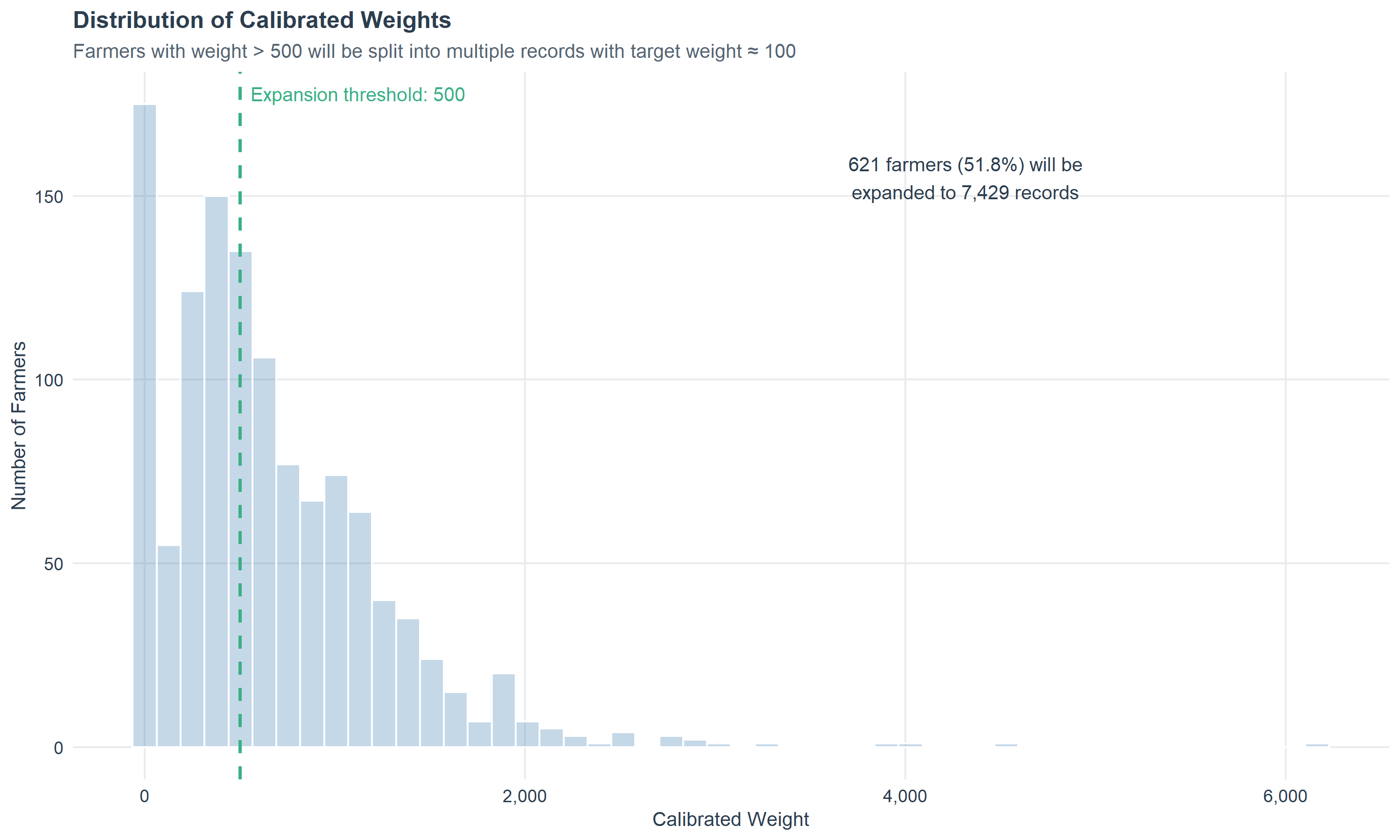
ImportantExpansion Strategy
Farmers with calibrated weight above the expansion threshold are split into multiple records, each with a target weight of approximately one fifth of the threshold. This brings the maximum weight down by an order of magnitude and smooths the large steps out of the distribution. A 3% standard deviation jitter is applied to base variables to introduce controlled variation among copies.
ImportantWhat the Adjustment Costs
The departmental targets are met exactly, and the adjustment needed to meet them is large. Individual weights are multiplied by factors spanning [0, 10.28], against the conventional working range of [0.3, 3.0]: 198 (16.5%) of records fall below 0.3 and 7 (0.6%) above 3.0.
The dispersion of the weights rises accordingly, with their coefficient of variation moving from 64.1% to 89.5% and a design effect of 1.801. This is the arithmetic consequence of the pre-calibration gap: the ENCOVI-to-MAGA production ratio runs from 0.5 to 10.12 across departments, so the weights carry the whole of that correction.
Final Validation
After expansion, jitter application, and re-calibration (to correct small jitter-induced bias), we verify the final dataset still matches MAGA targets.
| Final Validation: Expanded Dataset vs MAGA Targets | ||||||||||
| Weighted totals after expansion and re-calibration | ||||||||||
| Department |
Sample
|
Production (qq)
|
Land (mz)
|
|||||||
|---|---|---|---|---|---|---|---|---|---|---|
| Records | Households | Farmers | Final | MAGA | Ratio | Final | MAGA | Ratio | ||
| Alta Verapaz | 1,090 | 99 | 106,782 | 5,296,634 | 5,296,634 | 1.0000 | 252,979 | 252,979 | 1.0000 | |
| Baja Verapaz | 160 | 47 | 17,846 | 720,542 | 720,542 | 1.0000 | 40,233 | 40,233 | 1.0000 | |
| Chimaltenango | 468 | 84 | 46,641 | 1,065,264 | 1,065,264 | 1.0000 | 34,835 | 34,835 | 1.0000 | |
| Chiquimula | 493 | 97 | 50,738 | 1,518,844 | 1,518,844 | 1.0000 | 65,717 | 65,717 | 1.0000 | |
| El Progreso | 33 | 28 | 5,848 | 367,087 | 367,087 | 1.0000 | 20,283 | 20,283 | 1.0000 | |
| Escuintla | 179 | 28 | 18,216 | 528,828 | 528,828 | 1.0000 | 10,216 | 10,216 | 1.0000 | |
| Guatemala | 199 | 14 | 19,316 | 816,778 | 816,778 | 1.0000 | 28,939 | 28,939 | 1.0000 | |
| Huehuetenango | 851 | 64 | 82,011 | 4,023,703 | 4,023,703 | 1.0000 | 156,526 | 156,526 | 1.0000 | |
| Izabal | 390 | 85 | 37,863 | 1,254,753 | 1,254,753 | 1.0000 | 30,116 | 30,116 | 1.0000 | |
| Jalapa | 142 | 54 | 21,668 | 1,095,143 | 1,095,143 | 1.0000 | 40,300 | 40,300 | 1.0000 | |
| Jutiapa | 391 | 116 | 54,742 | 2,646,775 | 2,646,775 | 1.0000 | 86,098 | 86,098 | 1.0000 | |
| Petén | 376 | 73 | 42,446 | 10,658,142 | 10,658,142 | 1.0000 | 356,518 | 356,518 | 1.0000 | |
| Quetzaltenango | 272 | 33 | 25,551 | 2,580,710 | 2,580,710 | 1.0000 | 62,296 | 62,296 | 1.0000 | |
| Quiché | 893 | 74 | 86,830 | 5,171,702 | 5,171,702 | 1.0000 | 224,720 | 224,720 | 1.0000 | |
| Retalhuleu | 102 | 22 | 10,577 | 1,129,300 | 1,129,300 | 1.0000 | 29,346 | 29,346 | 1.0000 | |
| Sacatepéquez | 32 | 22 | 5,759 | 321,895 | 321,895 | 1.0000 | 12,495 | 12,495 | 1.0000 | |
| San Marcos | 553 | 46 | 54,490 | 2,538,994 | 2,538,994 | 1.0000 | 74,815 | 74,815 | 1.0000 | |
| Santa Rosa | 374 | 70 | 37,379 | 886,464 | 886,464 | 1.0000 | 23,071 | 23,071 | 1.0000 | |
| Sololá | 64 | 21 | 9,459 | 810,483 | 810,483 | 1.0000 | 24,550 | 24,550 | 1.0000 | |
| Suchitepéquez | 140 | 27 | 13,115 | 555,180 | 555,180 | 1.0000 | 11,689 | 11,689 | 1.0000 | |
| Totonicapán | 149 | 40 | 19,718 | 999,141 | 999,141 | 1.0000 | 42,234 | 42,234 | 1.0000 | |
| Zacapa | 78 | 55 | 16,478 | 774,130 | 774,130 | 1.0000 | 23,755 | 23,755 | 1.0000 | |
| Total | — | 7,429 | 1,199 | 783,474 | 45,760,490 | 45,760,490 | — | 1,651,732 | 1,651,732 | — |
| Ratio = Final / MAGA. Values of 1.0000 confirm exact calibration. Farmers = Weighted total of white maize farmers represented. Green highlight: both ratios within ±0.01% of target. |
||||||||||
Transformation Pipeline
| Dataset Transformation Pipeline | |||
| From ENCOVI sample to MAGA-calibrated expanded dataset | |||
| Stage | Records | Weight Range | Description |
|---|---|---|---|
| A. Input data (02_01 output) | 1,199 | [76, 2988] | Cleaned farmers from Script 02_01 with scaled ENCOVI weights (×1.95) |
| B. Weight calibration (MAGA) | 1,199 | [0, 6166] | Weights adjusted to match MAGA production and land totals by department |
| C. Record expansion | 7,429 | [0, 498] | High-weight farmers (>500) split into multiple records (target weight ≈100) |
| C. Jitter application | 7,429 | — | 3% SD jitter applied to base variables; derived variables recalculated |
| C. Re-calibration | 7,429 | [0, 524] | Second calibration pass to correct jitter-induced bias (~1%) |
| D. Final output | 7,429 | [0, 524] | Final dataset ready for segmentation modeling |
| Pipeline progresses from cleaned ENCOVI input through calibration, expansion with jitter, and re-calibration to the final dataset ready for segmentation modeling | |||
Summary
Key Findings
Initial discrepancies: Before calibration the ENCOVI-to-MAGA production ratio ranges from 0.5 to 10.12, with 13 of the 22 departments outside the [0.5, 2.0] range.
Calibration: Linear calibration brings both production and land area onto the MAGA departmental targets, with ratios at 1.0000.
Cost in weight dispersion: Meeting those targets moves the weight coefficient of variation from 64.1% to 89.5%, with a design effect of 1.801 and adjustment ratios spanning [0, 10.28].
Weight smoothing: Record expansion with controlled jitter removes the discontinuities from the distribution while holding the weighted totals, and a re-calibration pass corrects the small bias the non-negativity constraint introduces.
Application
The calibrated and expanded dataset provides:
- Representative farmer population — Weighted totals match official MAGA statistics for economic impact projections
- Smooth distributions — No artificial steps for threshold-based segmentation in farmer classification
- Internal consistency — Allocation coherence between total production and destination quantities preserved through the jitter procedure