| Base composite score distribution by segment | ||||||
| Pre-risk score. Expected ordering: Low > High > Mid > OPV/Criollo | ||||||
| Segment | N | Mean | SD | P25 | Median | P75 |
|---|---|---|---|---|---|---|
| Low | 313 | 88.9 | 7.5 | 85.5 | 91.5 | 94.3 |
| Mid | 411 | 65.2 | 7.8 | 59.4 | 65.3 | 70.3 |
| High | 1078 | 66.9 | 7.1 | 62.1 | 64.8 | 70.4 |
| OPV/Criollo | 5627 | 56.0 | 7.2 | 50.8 | 56.6 | 61.9 |
Likely Adopters Model Application
Module 2: Economic Impact
Why Apply the Likely Adopters Model?
The Likely Adopters model calibrated when determining its parameters encapsulates the structural relationship between farmer characteristics and adoption priority. Applying that model to a specific seed-by-subsidy combination produces a per-farmer dataset that ranks every farmer by expected adoption priority and assigns a continuous conversion curve governing how much of their white-maize land they would commit to biofortified seed at any national production coverage level.
This per-farmer dataset is the entry point for the M06 scenario engine, which evaluates the cohort of adopters at any chosen national production coverage and aggregates economic and nutrient outcomes accordingly. The application stage is therefore the bridge between farmer-level scoring and population-level scenario evaluation.
The figures presented here correspond to the baseline scenario combining the 2022 biofortified seed variety with the current subsidy regime. The calibrated model configuration is invariant across seed-by-subsidy combinations: the structural relationships between farmer characteristics and adoption priority depend on the joint distribution of farmer attributes, not on the magnitude of the projected economic benefit. The application stage runs the same calibrated configuration against each combination, producing a per-combination scored dataset.
Final Score Formulation
The final adoption score of farmer i is the base composite score net of the risk-aversion penalty:
\[ \text{adoption\_score}(i) = \text{score}_{\text{base}}(i) - w_R \cdot \text{penalty}_R(i) \]
where w_R is the calibrated risk weight and penalty_R(i) is the logistic risk-aversion penalty defined in Phase C. The base score score_base(i) is the weighted linear combination of the five component scores defined in Phase B.
The application proceeds in four sequential stages:
- Base composite score (Phase B) — applies the five scoring components defined by the calibrated configuration: segment priority, economic benefit, improvement potential, scale potential, and farmer profile.
- Risk-aversion penalty (Phase C) — computes an additive penalty reflecting structural reluctance based on four drivers (baseline yield, income-increment ratio, land entry size, projected income loss), combined through a logistic transformation.
- Ranking and continuous adoption (Phase D) — ranks farmers by the final score, derives each farmer’s entry production coverage point
p_entryinto the ranking, and prepares the per-farmer variables consumed by the M06 scenario engine through profile-specific sigmoid curves. - Cohort and validation diagnostics (Phase E) — reports the most informative downstream-facing diagnostics: cohort profile at five production coverage points, component score correlation matrix, calibrated specification summary, geographic distribution of priority adopters, and score distribution by department.
Phase A loads the per-farmer inputs — the economic impact data, the segmentation data, and the calibrated model configuration — joins them on the household and farmer identifier, and derives the per-farmer entry-size profile assignment (small, medium, large) that governs the scale-potential scoring component and the structural risk driver.
Phase B: Base Composite Score
The base composite score is the weighted linear combination of five components, each scored on a [0, 100] scale:
- Segment Priority — cardinal points per segment under the calibrated segment-priority scheme.
- Economic Benefit — percentile-based score over
income_increment, mapping farmers with higher projected economic gain to higher scores. - Improvement Potential — percentile-based score over
exp_total_per_mz_annual(inverse direction: lower per-area input expenditure indicates higher potential for productivity gains). - Scale Potential — percentile-based score over
land_entry_size(the per-farmer land commitment at the moment of entry into the ranking, equal toland_wtcorn × entry_coefwhereentry_coefdepends on profile). - Farmer Profile (Age) — three-axis parameterisation over
farmer_agegoverned bypeak_center,peak_width, and a profile shape, capturing the empirical observation that adoption propensity peaks in the productive-age range and declines towards both extremes.
The component weights are read from the calibrated model configuration. The full specification of all five components — variables, weights, and heuristic parameters — is reported in Phase E3 below.
Base Score Distribution by Segment
The base score distribution is read against the calibrated segment-priority ordering, before the risk-aversion correction is applied. The selected segment scheme assigns Low = 100, High = 85, Mid = 70 and OPV/Criollo = 45, so the expected ordering is Low > High > Mid > OPV/Criollo, with OPV/Criollo the non-hybrid segment.
The segment component carries a weight of 0.6 out of 1, which is why the composite base score follows the same ordering: mean scores of 88.9, 66.9, 65.2 and 56.0 respectively. The non-hybrid segment scoring last on adoption priority is consistent with the calibration anchors: these farmers hold the largest share of land and the largest yield increase, and the market composition data place their entry late in the coverage path.
Phase C: Risk-Aversion Penalty
The risk-aversion penalty discounts the base composite score of each farmer by an explicit measure of vulnerability to crop loss. Four drivers contribute to the penalty:
driver_yield— captures the per-farmer variability of expected yield against the departmental reference.driver_ratio— captures the marginal weight of the projected income increment relative to a baseline income proxy.driver_land— captures the per-farmer land commitment (with smaller plots interpreted as carrying greater relative risk from a single-season loss).driver_loss— captures the structural disincentive associated with a projected negative income increment.
The four drivers are linearly combined with the calibrated coefficients alpha_yield, alpha_ratio, alpha_land (sharing the unit weight budget set during calibration) and the structural coefficient alpha_loss = 1.0. The combined driver is transformed through a logistic function with slope β bounded in [0, 100], and the penalty is subtracted from the base score weighted by the calibrated w_R:
\[ \text{penalty}_R(i) = \frac{100}{1 + \exp\bigl(-\beta \cdot z_{\text{combo}}(i)\bigr)} \quad,\quad \text{adoption\_score}(i) = \text{score}_{\text{base}}(i) - w_R \cdot \text{penalty}_R(i) \]
The driver representation is selected from the calibrated variant held in the model configuration: either departmental z-scores (variant Z) or absolute values normalised through a P1–P99 weighted scaling (variant A). Only the calibrated variant is computed at application time, keeping the per-farmer dataset compact.
NoteStructural Loss Coefficient
The coefficient alpha_loss = 1.0 is held fixed by design across all configurations: it reflects the structural role of the projected-loss driver as a deterministic disincentive rather than a calibrated component. The remaining three coefficients share a unit weight budget calibrated against the empirical anchor set.
Risk Penalty Distribution by Segment
The penalty distribution is read against the qualitative behaviour the calibrated risk model is built to produce: a higher penalty among High-segment farmers, who commit more land and can face a negative income increment, than among Low-segment farmers. The means run 62.0 for High, 47.6 for OPV/Criollo, 44.3 for Mid and 40.0 for Low, which follows that ordering.
| Risk penalty distribution by segment (2022 seed) | ||||||
| Logistic penalty under the calibrated driver variant and risk weight | ||||||
| Segment | N | Mean | SD | P25 | Median | P75 |
|---|---|---|---|---|---|---|
| High | 1078 | 62.0 | 24.8 | 44.9 | 64.7 | 83.1 |
| OPV/Criollo | 5627 | 47.6 | 23.3 | 28.5 | 43.3 | 63.7 |
| Mid | 411 | 44.3 | 23.7 | 22.4 | 41.1 | 63.8 |
| Low | 313 | 40.0 | 19.5 | 24.2 | 35.8 | 55.2 |
Phase D: Ranking and Continuous Adoption
This phase ranks farmers by the final adoption score, derives each farmer’s entry production coverage point into the ranking, and prepares the per-farmer variables consumed by the M06 scenario engine.
Entry production coverage point. Farmers are sorted by adoption_score descending. The basal weight of each farmer is the product of total production and survey-calibrated weight; the cumulative basal weight divided by the universe total defines the entry production coverage point p_entry of each farmer, interpreted as the national production coverage level at which the farmer joins the ranking. By construction, p_entry ranges from 0 (top-ranked farmer) to just below 1 (last-ranked farmer with positive basal weight).
Adoption category. A presentation label is assigned for dashboard and report use based on the final score: A: Priority (score ≥ 80), B: High Potential (60 ≤ score < 80), C: Moderate (40 ≤ score < 60), D: Low (20 ≤ score < 40), and E: Not Recommended (score < 20). The category is a display label only; downstream economic computations operate on the continuous score, not on the category.
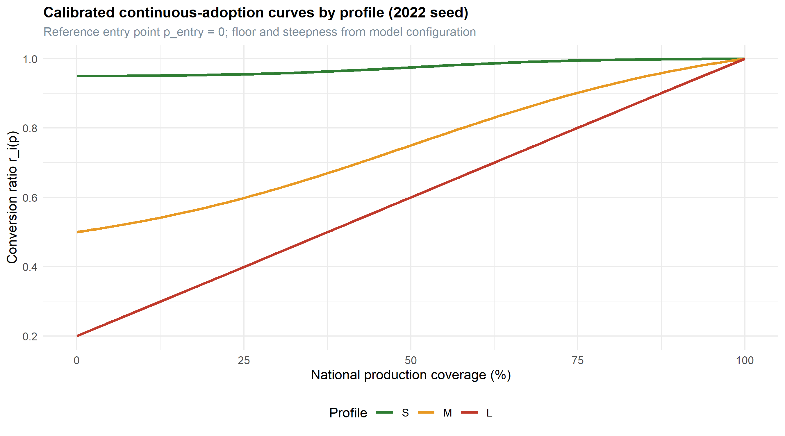
Continuous adoption curve. The per-farmer conversion ratio at national production coverage p follows a profile-specific sigmoid anchored at the farmer’s entry point:
\[ r_i(p) = \text{sigmoid\_curve}(p,\; p_{\text{entry},i},\; \text{floor}_{\text{profile}_i},\; k_{\text{profile}_i}) \]
where floor_profile is the conversion ratio achieved at the moment of entry and k_profile governs the rate at which the ratio approaches 1 as p advances. The figure below displays the curve shape for each profile under the calibrated parameters, evaluated for a representative entry point at p_entry = 0.
NoteProfile Differentiation in Adoption Pace
The three profile curves reflect the qualitative behavior calibrated against the empirical land trajectory: profile S (small) approaches near-full conversion almost immediately upon entry, profile M (medium) follows a sigmoid that saturates around mid-range production coverage levels, and profile L (large) accumulates gradually and reaches saturation only at high national production coverage. The shapes are entirely determined by the calibrated parameters; no per-farmer free parameters are introduced at the application stage.
Phase E: Cohort and Validation Diagnostics
This phase reports the most informative downstream-facing diagnostics. The cohort profile at five representative production coverage points provides a direct view of how the scoring engine populates the adopting cohort as national production coverage advances; the component correlation matrix verifies non-redundancy of the five scoring components; the calibrated specification summary reproduces the parameter set actually applied; and the geographic and per-department distributions characterise the spatial spread of priority adopters.
Cohort Profile at Five Production Coverage Points
For each national production coverage level p, the cohort is defined as the set of farmers whose entry production coverage is at or below p. Each cohort member contributes a per-farmer conversion ratio r_i(p) evaluated through the calibrated continuous-adoption curve; biofortified land and biofortified production are scaled by r_i(p). Income variables (current, projected, and increment) are reported as survey-weighted medians with interquartile range across the cohort, weighted by weight_calibrated × r_i(p). All monetary values are in Guatemalan Quetzales (Q).
| Cohort characteristics at five production coverage points (2022 seed) | |||||
| Survey-weighted medians [P25, P75] of the adopter cohort, disaggregated by segment. All monetary values in Quetzales (Q). | |||||
| OPV/Criollo | Low | Mid | High | Overall | |
|---|---|---|---|---|---|
| 10% | |||||
| Total Farmers | 4,292 | 25,512 | 14,340 | 27,214 | 71,358 |
| % Land | 0.41% | 1.73% | 0.57% | 1.03% | 3.74% |
| Land (mz) [Median, IQR] | 1.00 [0.95, 1.22] | 0.80 [0.38, 1.03] | 0.43 [0.22, 0.95] | 0.48 [0.12, 0.95] | 0.67 [0.25, 0.99] |
| Production (qq) [Median, IQR] | 33.2 [20.9, 37.5] | 26.3 [16.7, 47.8] | 19.1 [9.7, 28.5] | 21.5 [7.5, 47.3] | 23.7 [11.4, 41.0] |
| Net income — current (Q) [Median, IQR] | 4806.6 [3326.9, 7506.9] | 2466.7 [942.6, 7340.7] | 1701.7 [773.7, 3619.5] | 1285.6 [-87.1, 4337.8] | 2099.6 [599.6, 5640.7] |
| Net income — projected (Q) [Median, IQR] | 6844.4 [4755.9, 9114.4] | 3491.7 [1652.8, 9890.2] | 2100.9 [1078.5, 4094.6] | 1775.4 [318.3, 5649.6] | 2849.5 [1031.7, 7177.8] |
| Net income increment (Q) [Median, IQR] | 1502.1 [924.0, 2673.9] | 1093.2 [655.9, 2061.6] | 365.4 [109.0, 676.8] | 323.8 [105.5, 1227.9] | 698.3 [215.6, 1572.6] |
| 25% | |||||
| Total Farmers | 76,947 | 26,876 | 28,392 | 33,454 | 165,669 |
| % Land | 3.91% | 2.01% | 1.84% | 1.30% | 9.07% |
| Land (mz) [Median, IQR] | 0.56 [0.35, 0.98] | 0.80 [0.35, 1.04] | 0.54 [0.25, 0.95] | 0.36 [0.09, 0.95] | 0.55 [0.27, 0.97] |
| Production (qq) [Median, IQR] | 26.1 [17.9, 41.8] | 25.6 [16.3, 48.9] | 19.4 [9.7, 37.2] | 16.8 [6.6, 41.1] | 24.6 [13.2, 42.2] |
| Net income — current (Q) [Median, IQR] | 3199.9 [1796.8, 5473.4] | 2341.9 [942.5, 7309.0] | 1457.8 [338.7, 3953.4] | 1127.6 [-89.6, 4040.7] | 2492.4 [942.7, 5223.0] |
| Net income — projected (Q) [Median, IQR] | 4476.8 [2751.6, 7561.9] | 3447.6 [1643.8, 9921.1] | 1917.9 [611.7, 4248.8] | 1439.7 [216.7, 5084.2] | 3539.6 [1501.3, 7033.8] |
| Net income increment (Q) [Median, IQR] | 1186.1 [852.3, 2122.8] | 1096.7 [609.2, 2070.1] | 268.5 [104.4, 719.0] | 231.8 [26.7, 1024.7] | 926.6 [346.1, 1664.3] |
| 50% | |||||
| Total Farmers | 301,221 | 29,426 | 31,970 | 47,334 | 409,950 |
| % Land | 18.36% | 2.52% | 2.87% | 1.72% | 25.47% |
| Land (mz) [Median, IQR] | 0.74 [0.36, 1.04] | 0.80 [0.36, 1.07] | 0.58 [0.26, 1.01] | 0.24 [0.08, 0.92] | 0.68 [0.31, 1.02] |
| Production (qq) [Median, IQR] | 22.1 [12.6, 43.8] | 25.7 [15.2, 54.9] | 20.8 [10.5, 40.7] | 11.8 [6.6, 36.4] | 21.4 [12.2, 43.7] |
| Net income — current (Q) [Median, IQR] | 2210.3 [874.8, 4775.4] | 2341.9 [942.5, 7377.4] | 1360.7 [95.2, 3799.3] | 1206.8 [101.5, 3134.0] | 2022.4 [765.6, 4635.6] |
| Net income — projected (Q) [Median, IQR] | 3181.8 [1492.7, 6668.5] | 3290.5 [1487.2, 9729.2] | 1733.3 [364.3, 4140.6] | 1391.2 [277.0, 3537.7] | 2822.1 [1232.3, 6391.4] |
| Net income increment (Q) [Median, IQR] | 919.2 [483.1, 1879.7] | 1061.5 [544.4, 2112.3] | 289.1 [100.2, 893.7] | 80.7 [-93.8, 518.0] | 802.7 [358.6, 1720.4] |
| 75% | |||||
| Total Farmers | 431,252 | 31,487 | 35,569 | 71,911 | 570,219 |
| % Land | 36.47% | 3.01% | 3.74% | 2.69% | 45.91% |
| Land (mz) [Median, IQR] | 0.92 [0.44, 1.25] | 0.78 [0.35, 1.09] | 0.57 [0.26, 1.02] | 0.25 [0.09, 0.88] | 0.83 [0.35, 1.16] |
| Production (qq) [Median, IQR] | 21.9 [12.6, 52.1] | 26.0 [14.6, 57.2] | 20.7 [10.5, 40.7] | 12.7 [7.3, 41.1] | 21.2 [11.4, 49.9] |
| Net income — current (Q) [Median, IQR] | 2041.7 [723.4, 5172.5] | 2330.6 [942.5, 7320.8] | 1430.3 [157.0, 3677.9] | 1572.4 [315.0, 3798.6] | 1948.1 [659.9, 4960.9] |
| Net income — projected (Q) [Median, IQR] | 2911.6 [1240.1, 7482.9] | 3182.1 [1393.8, 9522.8] | 1735.9 [375.5, 4106.4] | 1488.8 [307.6, 3772.0] | 2670.9 [1046.7, 6720.6] |
| Net income increment (Q) [Median, IQR] | 871.1 [389.9, 2270.3] | 1048.3 [508.3, 2177.5] | 268.0 [95.5, 807.3] | -88.8 [-278.1, 238.6] | 709.2 [257.7, 1877.7] |
| 100% | |||||
| Total Farmers | 594,812 | 32,354 | 44,169 | 112,140 | 783,474 |
| % Land | 87.06% | 3.43% | 4.71% | 4.80% | 100.00% |
| Land (mz) [Median, IQR] | 1.00 [0.48, 2.00] | 0.78 [0.35, 1.09] | 0.50 [0.23, 1.00] | 0.29 [0.11, 0.97] | 0.91 [0.35, 1.50] |
| Production (qq) [Median, IQR] | 21.1 [11.0, 52.6] | 26.2 [14.7, 62.8] | 20.4 [10.0, 39.4] | 17.2 [8.4, 46.4] | 20.9 [10.5, 51.7] |
| Net income — current (Q) [Median, IQR] | 1864.1 [557.3, 5040.3] | 2330.6 [942.5, 7320.8] | 1500.6 [252.3, 3883.0] | 2058.0 [675.3, 5021.2] | 1883.9 [567.9, 5040.3] |
| Net income — projected (Q) [Median, IQR] | 2554.8 [827.1, 6849.1] | 3186.7 [1396.0, 9533.7] | 1714.0 [247.3, 4067.3] | 1659.5 [354.5, 4275.9] | 2381.3 [718.8, 6294.9] |
| Net income increment (Q) [Median, IQR] | 686.8 [220.4, 1989.5] | 1068.6 [511.0, 2273.1] | 190.9 [21.8, 677.3] | -260.3 [-743.5, 25.8] | 534.9 [46.2, 1581.0] |
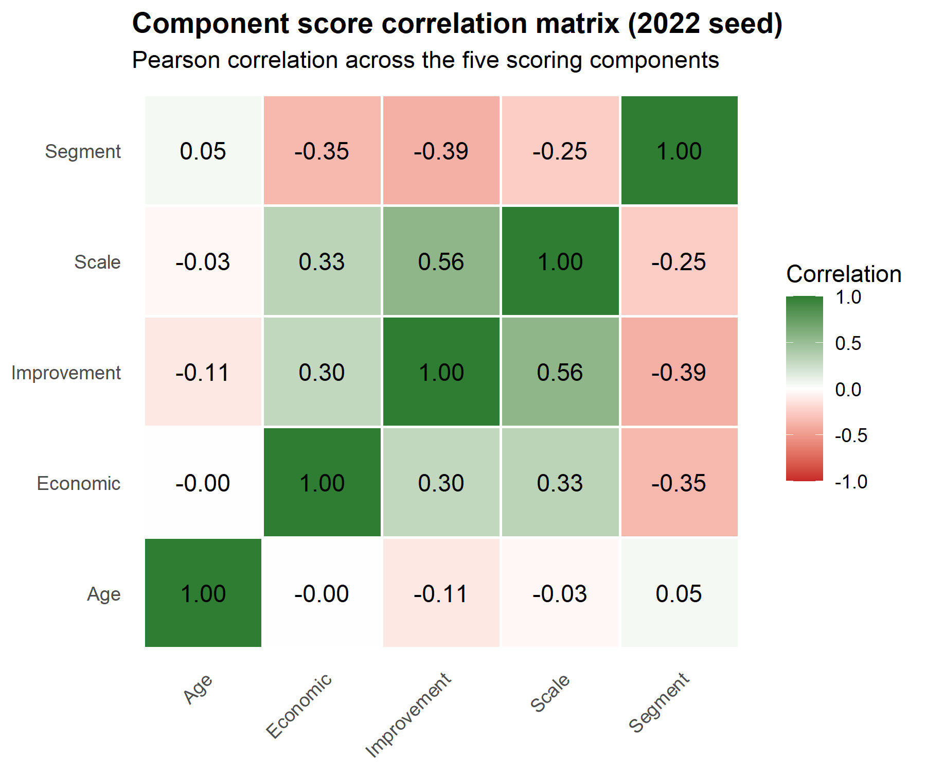
Component Score Correlation Matrix
The five component scores should capture distinct dimensions of farmer characteristics. The correlation matrix verifies component independence: low pairwise correlations indicate non-redundant signals, while high correlations would suggest that two components carry overlapping information and the composite weighting is double-counting.
Calibrated Model Specification
The applied model specification is summarised below, reading directly from the model configuration artefact produced by 05_05. This table is the auditable counterpart of the determination summary produced at calibration time.
| Applied Likely Adopters model specification (2022 seed) | |
| Parameters read from the calibration artefact produced by 05_05 | |
| Parameter | Value |
|---|---|
| Metadata | |
| Calibration seed/subsidy | s22 + sub00 |
| Calibration date | 2026-08-05 |
| Scoring | |
| Segment scheme | lhm_shallow (Low=100, OPV=45, Mid=70, High=85) |
| Component weights | seg=0.6, econ=0.162, impr=0.088, scale=0.08, age=0.07 |
| Economic breakpoints | (0.2, 0.4, 0.6) |
| Improvement breakpoints | (0.3, 0.6, 0.8, 0.95) |
| Scale breakpoints | (0.25, 0.5, 0.75) |
| Age parameters | peak_center=55, peak_width=10, profile=neutral_edges |
| Risk | |
| Driver variant | z |
| Driver coefficients (yield, ratio, land) | (0, 0.1, 0.9) |
| Logistic slope β | 1.00 |
| Risk weight w_R | 0.40 |
| Continuous | |
| Profile cutoffs (S/M, M/L) (mz) | (1.25, 3) |
| Profile floors (S, M, L) | (0.95, 0.5, 0.2) |
| Profile steepness (k_S, k_M, k_L) | (8, 4, 0.5) |
| Entry size | |
| Entry cutoffs (S/M, M/L) (mz) | (1.5, 7) |
| Entry coefficients (S, M, L) | (0.95, 0.5, 0.2) |
Geographic Distribution of Priority Adopters
The geographic distribution reports the share of priority adopters (categories A and B) by department, weighted by weight_calibrated. The expanded farmer counts use survey weights to represent the national population.
| Geographic distribution of priority adopters (2022 seed) | ||||
| Survey-weighted counts of farmers in categories A and B | ||||
| Department | Total farmers (weighted) | Priority farmers (weighted) | % Priority within dept. | % Share of national priority |
|---|---|---|---|---|
| Alta Verapaz | 106,782 | 8,409 | 7.87 | 15.41 |
| Petén | 42,446 | 5,865 | 13.82 | 10.75 |
| Quiché | 86,830 | 4,723 | 5.44 | 8.66 |
| Izabal | 37,863 | 4,620 | 12.20 | 8.47 |
| Huehuetenango | 82,011 | 4,411 | 5.38 | 8.08 |
| Jutiapa | 54,742 | 3,876 | 7.08 | 7.10 |
| Santa Rosa | 37,379 | 3,870 | 10.35 | 7.09 |
| Escuintla | 18,216 | 3,074 | 16.87 | 5.63 |
| Chimaltenango | 46,641 | 2,933 | 6.29 | 5.37 |
| San Marcos | 54,490 | 2,425 | 4.45 | 4.44 |
| Retalhuleu | 10,577 | 2,413 | 22.81 | 4.42 |
| Chiquimula | 50,738 | 1,476 | 2.91 | 2.70 |
| Suchitepéquez | 13,115 | 1,347 | 10.27 | 2.47 |
| Sololá | 9,459 | 911 | 9.63 | 1.67 |
| El Progreso | 5,848 | 906 | 15.49 | 1.66 |
| Zacapa | 16,478 | 856 | 5.19 | 1.57 |
| Quetzaltenango | 25,551 | 722 | 2.82 | 1.32 |
| Baja Verapaz | 17,846 | 568 | 3.18 | 1.04 |
| Sacatepéquez | 5,759 | 423 | 7.35 | 0.78 |
| Totonicapán | 19,718 | 383 | 1.94 | 0.70 |
| Jalapa | 21,668 | 355 | 1.64 | 0.65 |
| Guatemala | 19,316 | 0 | 0.00 | 0.00 |
Score Distribution by Department
The departmental score distribution reports the survey-weighted distribution of the final adoption score across departments. The percentile summary surfaces geographic heterogeneity in adoption potential beyond what the priority-category summary alone reveals.
| Final adoption score distribution by department (2022 seed) | |||||
| Survey-weighted distribution of the final adoption score | |||||
| Department | Farmers (weighted) | Mean | P25 | Median | P75 |
|---|---|---|---|---|---|
| Petén | 42,446 | 45.2 | 38.5 | 47.9 | 54.4 |
| Quetzaltenango | 25,551 | 43.1 | 36.0 | 46.1 | 48.9 |
| Retalhuleu | 10,577 | 45.6 | 35.4 | 42.8 | 54.1 |
| Alta Verapaz | 106,782 | 41.0 | 36.3 | 42.4 | 46.0 |
| Escuintla | 18,216 | 41.2 | 28.5 | 41.7 | 51.5 |
| Zacapa | 16,478 | 41.1 | 37.7 | 41.3 | 45.1 |
| Sololá | 9,459 | 40.7 | 38.3 | 41.3 | 45.2 |
| Jalapa | 21,668 | 38.7 | 35.8 | 41.2 | 44.0 |
| Jutiapa | 54,742 | 41.6 | 36.4 | 40.9 | 47.2 |
| Baja Verapaz | 17,846 | 36.9 | 34.3 | 40.9 | 44.5 |
| Quiché | 86,830 | 39.8 | 34.5 | 40.7 | 44.0 |
| Suchitepéquez | 13,115 | 41.7 | 33.7 | 40.5 | 49.7 |
| Huehuetenango | 82,011 | 38.4 | 32.1 | 40.1 | 44.9 |
| El Progreso | 5,848 | 41.7 | 34.8 | 40.0 | 47.2 |
| Chiquimula | 50,738 | 36.9 | 33.3 | 39.6 | 43.2 |
| Izabal | 37,863 | 41.0 | 35.3 | 39.3 | 46.6 |
| Santa Rosa | 37,379 | 40.5 | 32.0 | 39.1 | 47.7 |
| Totonicapán | 19,718 | 37.0 | 34.0 | 38.8 | 42.6 |
| San Marcos | 54,490 | 38.3 | 33.8 | 38.3 | 43.3 |
| Guatemala | 19,316 | 36.9 | 36.0 | 38.2 | 42.8 |
| Sacatepéquez | 5,759 | 36.1 | 25.7 | 37.0 | 44.2 |
| Chimaltenango | 46,641 | 37.0 | 30.5 | 36.2 | 43.0 |
Summary
From Per-Farmer Score to Scenario Engine
The application stage converts the calibrated Likely Adopters configuration into a per-farmer dataset that the M06 scenario engine consumes directly. Three artefacts are produced and propagated downstream:
- Per-farmer adoption score — final value combining the base composite score with the risk-aversion penalty, used to rank farmers from most to least likely adopter.
- Entry production coverage point — cumulative basal weight divided by the universe total, defining at which national production coverage each farmer joins the ranking.
- Profile assignment and conversion curve parameters — small, medium, or large profile per farmer, each with its calibrated floor and steepness governing the per-farmer conversion ratio at any chosen national production coverage level.
Invariance Across Seed-by-Subsidy Combinations
The calibrated model configuration is structurally invariant across the nine seed-by-subsidy combinations produced by the economic impact calculation. The application script runs the same calibrated configuration against each combination, producing a per-combination scored dataset that preserves the relative ranking of farmers while reflecting the magnitude of the projected economic benefit in the underlying income_increment variable.
What the Diagnostics Show
The diagnostics in the final section report the applied model against its expected qualitative behaviour. The base score ordering recovers the calibrated segment scheme, Low > High > Mid > OPV/Criollo. The risk penalty is highest in the High segment, at a mean of 62.0 against 40.0 in Low, which matches the structural reluctance the driver is built to represent. The component score correlations stay modest enough to keep the five components non-redundant. The cohort profile at five production coverage points reproduces the anchor pattern of the New Seed market composition matrix used during calibration: at 10% national coverage the cohort is drawn mostly from the Low and High segments, and the non-hybrid segment enters later, reaching 87.1% of biofortified land only at full coverage.