Farmer Segmentation

Module 2: Economic Impact

Why Segment Farmers?

ENCOVI does not directly ask farmers whether they use non-hybrid varieties (locally known as OPV — open-pollinated varieties — or criollo, traditional landraces) or commercial hybrid seed. Yet this distinction is fundamental for assessing the economic impact of adopting biofortified maize seeds:

Non-hybrid farmers stand to gain most from biofortified seed adoption, since theirs are the largest yield increases
Hybrid farmers already use improved seed and may see smaller or negative yield changes when switching to biofortified varieties

We therefore infer seed technology from observable agricultural behaviours, and segment farmers accordingly so that each segment receives its own economic parameters.

Target Segments

These are the target segments of behaviour for the farmers:

The segment label `OPV/Criollo` is the value carried by the dataset and is retained throughout the tables and figures. OPV stands for open-pollinated varieties and criollo for traditional landraces; both are non-hybrid seed.
Segment	Description	Seed Behavior
OPV/Criollo	Non-hybrid farmers	Zero or near-zero seed expenditure
Low	Low technology adoption	Minimal purchased seed investment
Mid	Moderate adoption	Intermediate seed investment
High	High technology adoption	Highest seed investment, premium hybrid varieties

The Segmentation Challenge

A single variable, seed expenditure on its own, does not identify the segment:

High seed expenditure may indicate hybrid use or inefficient purchasing, where farmers buy expensive seed and obtain low yields, which points to a variety poorly matched to local conditions or to agronomic management that dilutes the value of the purchased seed
Low seed expenditure may indicate non-hybrid use or subsidized access to hybrid seed
Yield on its own confounds genetics with soil quality and management practices

We need a multidimensional approach that combines multiple behavioral signals while controlling for regional heterogeneity.

Departmental Z-Score Standardization

Agricultural conditions vary dramatically across Guatemala’s departments. Direct comparison of raw values would confound regional effects with technology choices.

Solution: Calculate z-scores relative to departmental means, measuring each farmer’s position within their local agricultural context.

Table 1: Departmental reference statistics for z-score calculation

Departmental Reference Statistics for Z-Score Calculation. Weighted means and standard deviations (n = 534 hybrid-potential households)
Department	Yield (qq/mz)		Seed Expenditure (Q/mz)		Sample
Departmental Reference Statistics for Z-Score Calculation
Weighted means and standard deviations (n = 534 hybrid-potential households)
Department	Mean	SD	Mean	SD	Households	% Total
Jutiapa	29.8	21.3	705	938	69	12.9%
Santa Rosa	31.8	24.6	711	922	47	8.8%
Petén	23.8	18.6	305	564	43	8.1%
Izabal	32.0	32.4	625	1,025	38	7.1%
Chiquimula	29.8	18.4	278	269	38	7.1%
Huehuetenango	37.6	34.4	332	656	32	6.0%
Alta Verapaz	35.7	24.9	319	665	31	5.8%
Quiché	32.5	30.6	388	609	29	5.4%
Zacapa	34.4	26.6	303	322	26	4.9%
Escuintla	26.4	33.9	1,111	1,470	24	4.5%
Jalapa	19.3	16.7	119	149	21	3.9%
Retalhuleu	34.7	36.5	497	417	19	3.6%
Suchitepéquez	46.4	27.7	793	798	17	3.2%
Chimaltenango	18.2	23.0	218	381	16	3.0%
Quetzaltenango	49.7	18.8	671	627	16	3.0%
Baja Verapaz	43.8	39.1	404	524	14	2.6%
Totonicapán	34.2	20.7	179	222	13	2.4%
El Progreso	25.1	27.1	322	847	11	2.1%
Sacatepéquez	30.7	38.2	90	165	10	1.9%
Sololá	40.3	31.9	153	150	10	1.9%
San Marcos	31.3	13.6	147	161	7	1.3%
Guatemala	33.1	17.5	151	87	3	0.6%
Source: ENCOVI 2023 agricultural module, MAGA-calibrated weights. Statistics calculated using survey-weighted means and variances.

Regional Heterogeneity

Yield and seed expenditure vary substantially across departments. Z-score standardization controls for these regional differences, enabling meaningful cross-departmental comparison of farmer behavior.

Dual-Framework Segmentation Approach

Two independent segmentation approaches are applied and validated against each other through their convergence. Agreement between an unsupervised method and a rule-based one is evidence that the resulting groups sit in the data rather than in either procedure.

Framework 1: PAM Clustering with Linear Discriminant Analysis (LDA) Validation

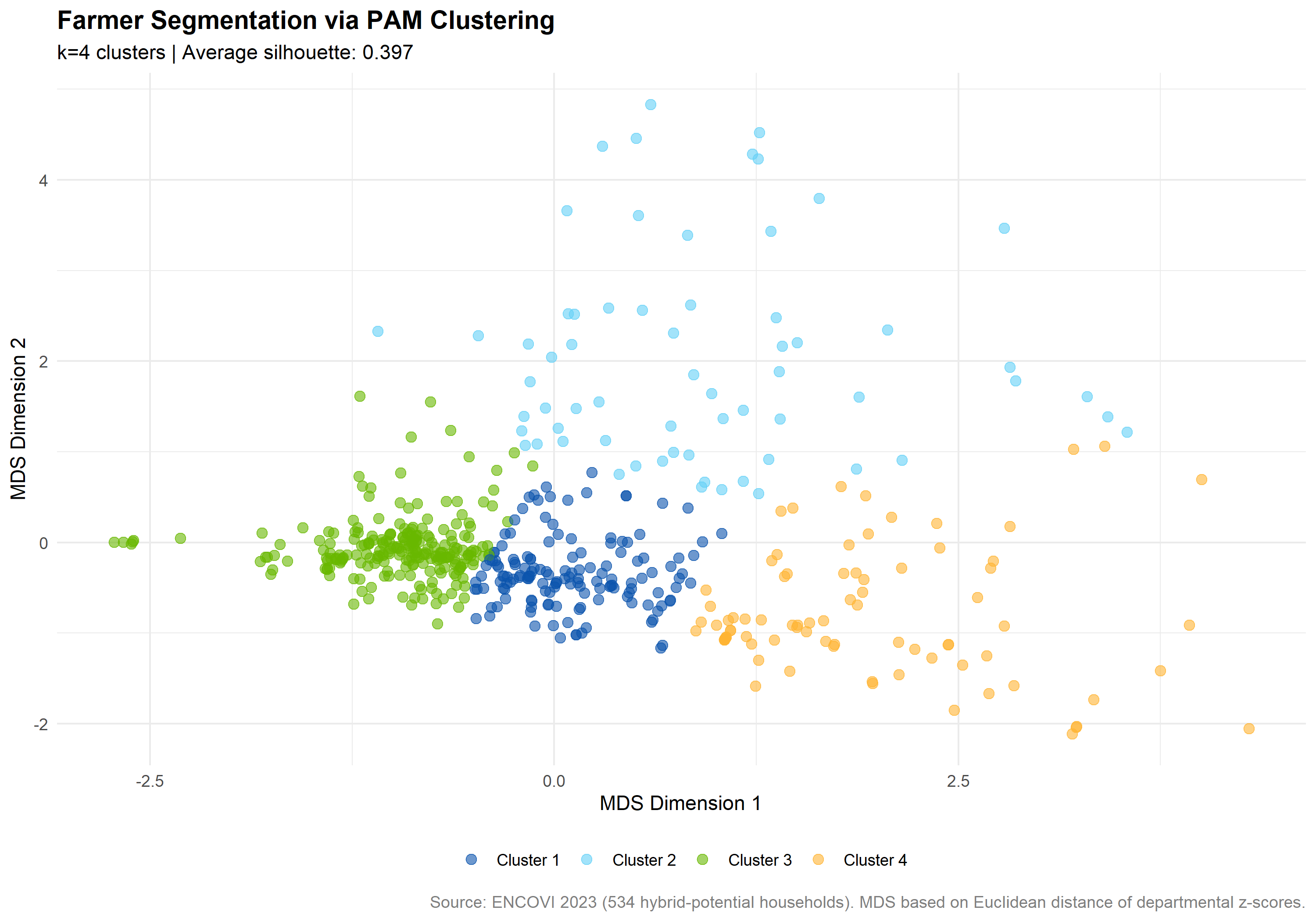
Partitioning Around Medoids (PAM) discovers natural groupings in the bidimensional z-score space through unsupervised learning. Unlike k-means, PAM uses actual data points (medoids) as cluster centers, providing interpretable farmer prototypes.

As we have 4 target farmer segments/groups, we are going to aim toward k = 4 clusters.

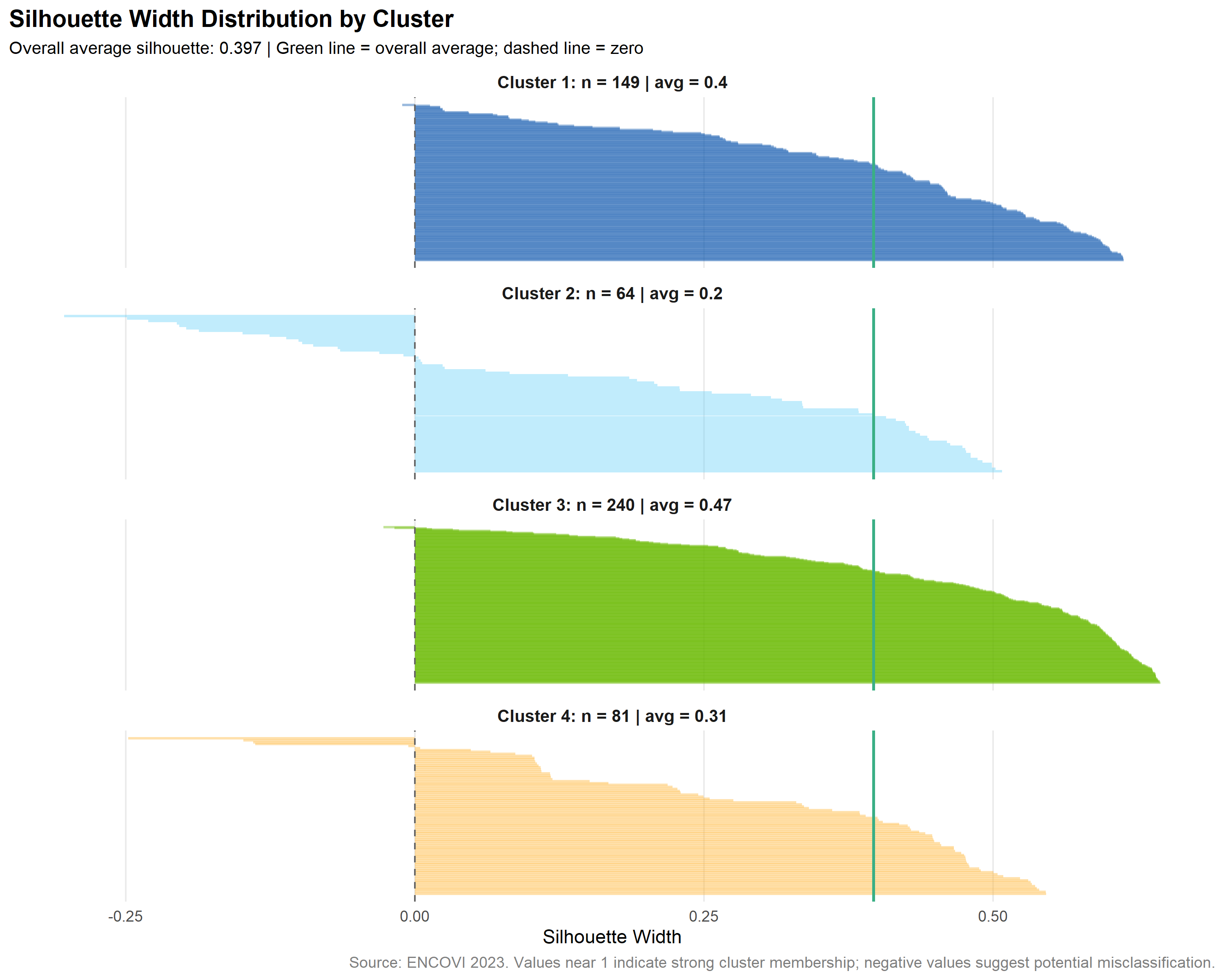
Cluster Quality: Silhouette Analysis

Silhouette analysis measures how well each observation fits within its assigned cluster versus neighboring clusters. Values range from -1 (poor fit) to +1 (strong fit).

Scatter chart of MDS Dimension 1 on the x-axis against MDS Dimension 2 on the y-axis, with points colored by their assigned PAM cluster (four clusters). Points fall into four visually separable groupings, showing that farmers form distinct behavioral clusters in the standardized yield and seed-expenditure space rather than a single continuous mass. — Figure 1: PAM clustering visualization in MDS space (k=4 clusters)

Silhouette plot with four stacked panels, one per cluster, showing a horizontal bar for each farmer whose length is its silhouette width along the x-axis. A dashed line marks zero and a solid green line marks the overall average width. Most bars extend to the right of zero, indicating generally positive membership, while a small number of negative bars flag potentially misclassified farmers. — Figure 2: Silhouette width distribution by cluster

Cluster Quality Assessment

Average silhouette coefficient = 0.397. Values above 0.25 indicate reasonable cluster structure and values above 0.50 strong structure, which places this result in the reasonable range.

LDA Variable Importance

Linear Discriminant Analysis (LDA) quantifies how much each variable contributes to separating the PAM clusters. These empirically-derived importance weights inform the final scoring system.

Table 2: Variable importance from Linear Discriminant Analysis

Variable Importance from Linear Discriminant Analysis. Based on sum of absolute coefficients across discriminant functions
Variable	Importance (%)	Cumulative (%)
Variable Importance from Linear Discriminant Analysis
Based on sum of absolute coefficients across discriminant functions
Seed expenditure z-score (departmental)	50.4	50.4
Yield z-score (departmental)	49.6	100.0
Source: LDA on k=4 PAM clusters (n=534 households). Importance = sum of \|coefficients\| across LD1 and LD2.

LDA-Derived Weights

The LDA analysis reveals that seed expenditure and yield contribute nearly equally to cluster separation. These empirically-derived weights form the foundation of the scoring system, ensuring variable weights are data-driven rather than arbitrary.

PAM Cluster Characteristics

Table 3: Cluster characteristics from PAM segmentation (Framework 1)

PAM Cluster Characteristics (Framework 1). Survey-weighted means for 534 hybrid-potential households
Cluster	Sample		Z-Scores		Original Scale
PAM Cluster Characteristics (Framework 1)
Survey-weighted means for 534 hybrid-potential households
Cluster	Households	% Population	Yield (z)	Seed Exp (z)	Yield (qq/mz)	Seed Exp (Q/mz)	Land (mz)
1	149	28.2%	+0.31	−0.30	38.3	258	2.6
2	64	13.5%	+0.28	+2.03	38.4	1,651	0.9
3	240	47.0%	−0.75	−0.40	11.8	205	2.4
4	81	11.3%	+2.01	−0.01	81.7	503	2.0
Source: ENCOVI 2023. PAM clustering (k=4) on departmental z-scores.

Framework 2: Quadrant Segmentation

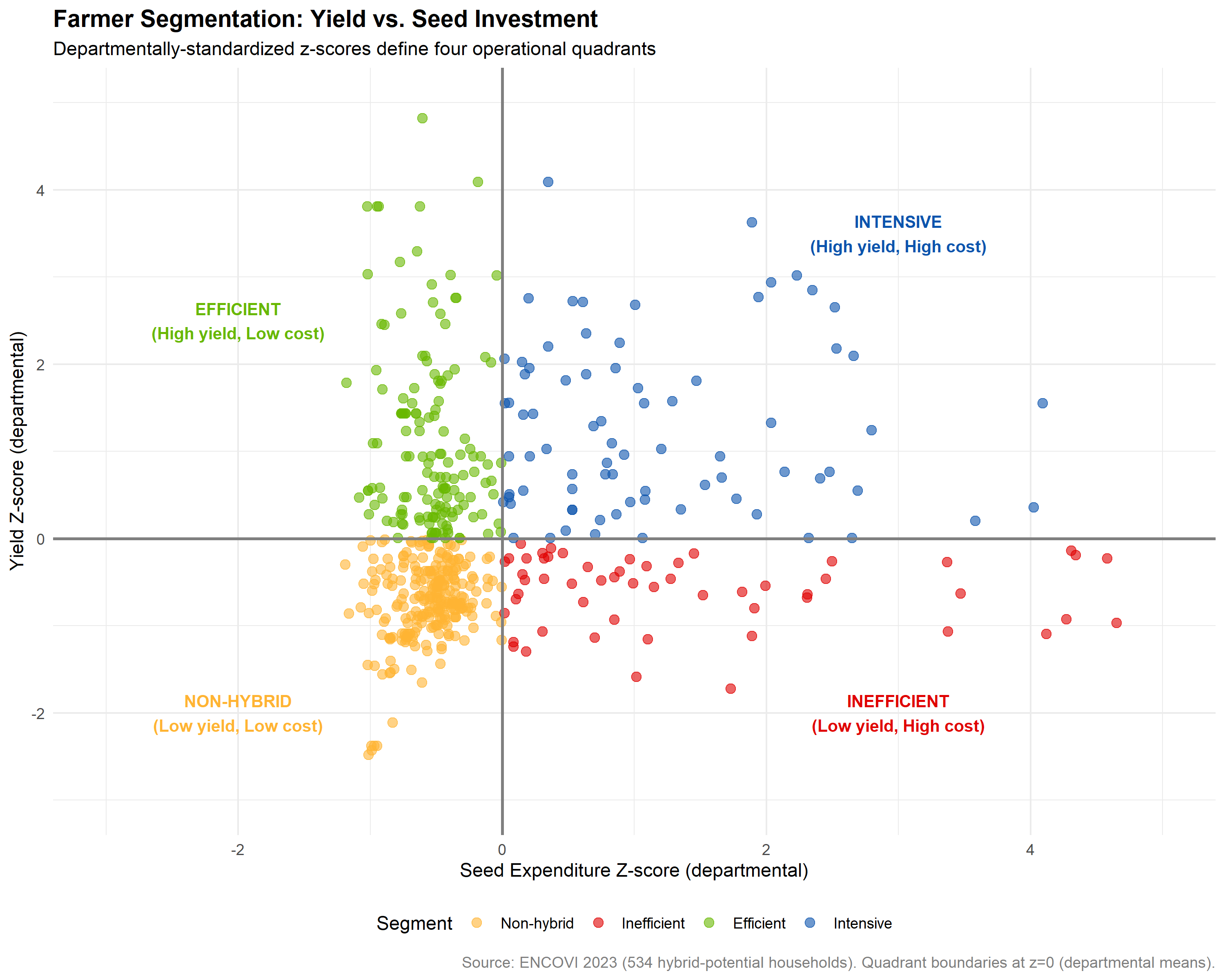
Theory-driven boundaries at z-score = 0 (departmental means) create four quadrants with clear economic interpretations. This deterministic approach provides transparency and reproducibility.

Scatter chart of seed expenditure z-score on the x-axis against yield z-score on the y-axis, with reference lines at zero dividing the plane into four quadrants. Points are colored by segment and each quadrant is labeled: Efficient (high yield, low cost), Intensive (high yield, high cost), Non-hybrid (low yield, low cost) and Inefficient (low yield, high cost). Points cluster within their labeled quadrants, showing that the theory-driven boundaries at the departmental means separate distinct farmer profiles. — Figure 3: Farmer segmentation in bidimensional z-score space (Framework 2)

Quadrant Interpretation

Each quadrant represents a distinct agricultural profile:

Non-hybrid (orange): below-average yield and below-average seed expenditure, the profile of non-hybrid seed users
Inefficient (red): below-average yield with above-average seed expenditure, consistent with hybrid users obtaining low returns
Efficient (green): above-average yield with below-average seed expenditure
Intensive (blue): above-average yield and above-average seed expenditure, the profile of hybrid adopters investing in technology

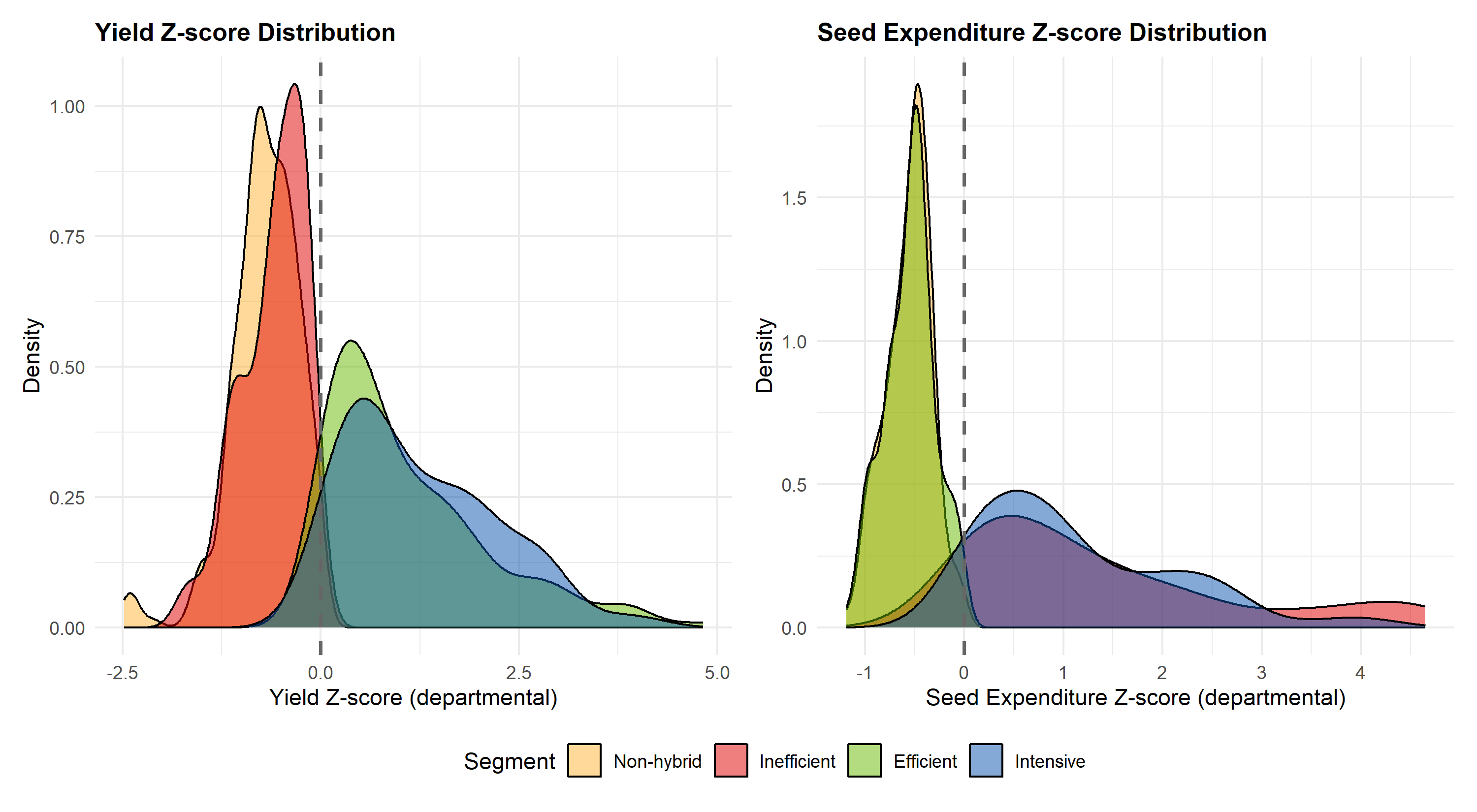
Z-Score Distributions by Segment

Density plots showing the distribution of yield and seed expenditure z-scores within each quadrant segment. The vertical dashed lines at z=0 mark the quadrant boundaries.

Two density plots side by side, sharing a segment color legend. The left panel shows the distribution of yield z-scores and the right panel the distribution of seed expenditure z-scores, each with one overlaid density curve per quadrant segment and a dashed line at zero. The segment curves peak on opposite sides of zero, confirming that the quadrants occupy distinct ranges along both the yield and seed-expenditure dimensions. — Figure 4: Z-score distributions by quadrant segment (Framework 2)

Quadrant Segment Characteristics

Table 4: Quadrant segment characteristics (Framework 2)

Quadrant Segment Characteristics (Framework 2). Survey-weighted means for 534 hybrid-potential households
Segment	Sample		Z-Scores		Original Scale
Quadrant Segment Characteristics (Framework 2)
Survey-weighted means for 534 hybrid-potential households
Segment	Households	% Population	Yield (z)	Seed Exp (z)	Yield (qq/mz)	Seed Exp (Q/mz)	Land (mz)
Non-hybrid	254	46.5%	−0.68	−0.50	13.1	144	2.6
Inefficient	55	13.4%	−0.56	+1.26	18.4	1,262	1.2
Efficient	147	23.6%	+0.88	−0.49	52.2	137	2.8
Intensive	78	16.5%	+1.12	+1.10	59.8	1,093	1.2
Source: ENCOVI 2023. Quadrant segments defined by z-score signs (boundary at z=0).

Framework Convergence Analysis

Cross-tabulation of PAM cluster assignments (Framework 1) against quadrant segments (Framework 2) validates that both approaches identify similar underlying structure.

Table 5: Framework convergence: PAM clusters vs quadrant segments

Framework Convergence: PAM Clusters vs Quadrant Segments. Cross-tabulation of household assignments (n = 534) | Agreement rate: 78.7%
PAM Cluster	Quadrant Segments (Framework 2)				Total
Framework Convergence: PAM Clusters vs Quadrant Segments
Cross-tabulation of household assignments (n = 534) \| Agreement rate: 78.7%
PAM Cluster	Non-hybrid	Inefficient	Efficient	Intensive	Total
1	33	8	92	16	149
2	0	28	0	36	64
3	221	19	0	0	240
4	0	0	55	26	81
Note: Cluster 3 ↔︎ Non-hybrid (92%), Cluster 4 ↔︎ Efficient (72%), Cluster 2 ↔︎ Intensive (56%). Cluster 1 spans the two above-average-yield quadrants.

Reading the Cross-Tabulation

The two frameworks agree on 78.7% of households. The correspondence is strongest at the non-hybrid end, where 221 of 240 households in PAM cluster 3 fall in the Non-hybrid quadrant. It is weaker among the hybrid-potential clusters: cluster 4 maps to Efficient for 55 of 81 households, cluster 2 to Intensive for 36 of 64, and cluster 1 divides between the two above-average-yield quadrants, which is why the agreement calculation counts both as a match for that cluster.

The segment that matters most for the economic projection, the non-hybrid one, is the one the two frameworks separate most cleanly.

Empirical Justification for Variable Selection

The scoring system includes four variables: yield z-score (primary), seed expenditure z-score (primary), poverty level (modulator), and land ownership (modulator). The following correlation analyses justify these selections.

Primary Variables: Yield and Seed Expenditure

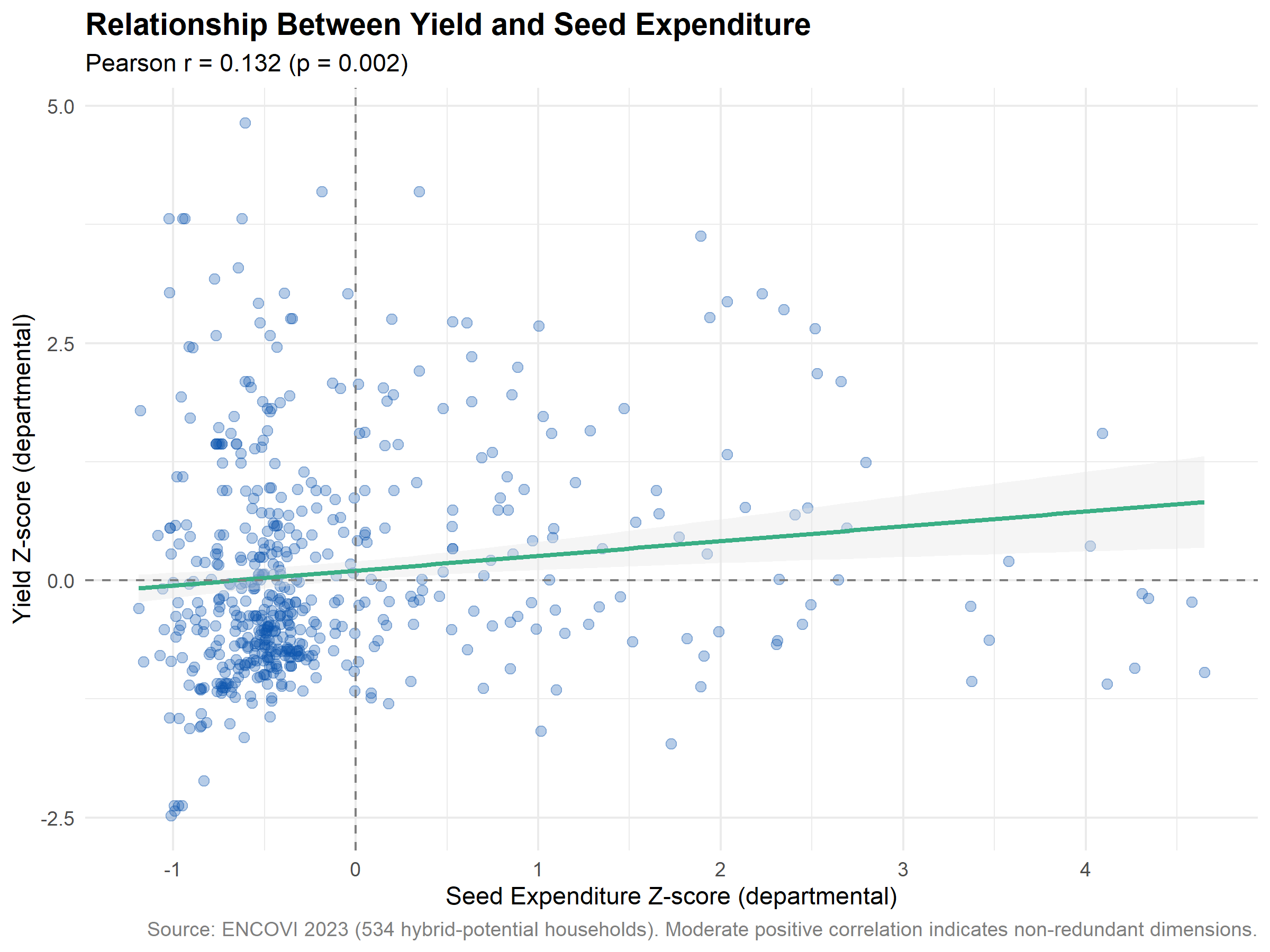
Scatter chart of seed expenditure z-score on the x-axis against yield z-score on the y-axis, with dashed reference lines at zero and an overlaid linear fit with a shaded confidence band. The fitted line slopes gently upward, indicating a moderate positive correlation, so the two variables capture related but non-redundant dimensions of agricultural performance. — Figure 5: Correlation between yield and seed expenditure z-scores

Non-Redundant Dimensions

The moderate positive correlation (r = 0.132) between yield and seed expenditure z-scores indicates that these variables capture distinct dimensions of agricultural performance. If they were highly correlated, using both would provide redundant information.

Stratified Analysis: Poverty Level as Modulator

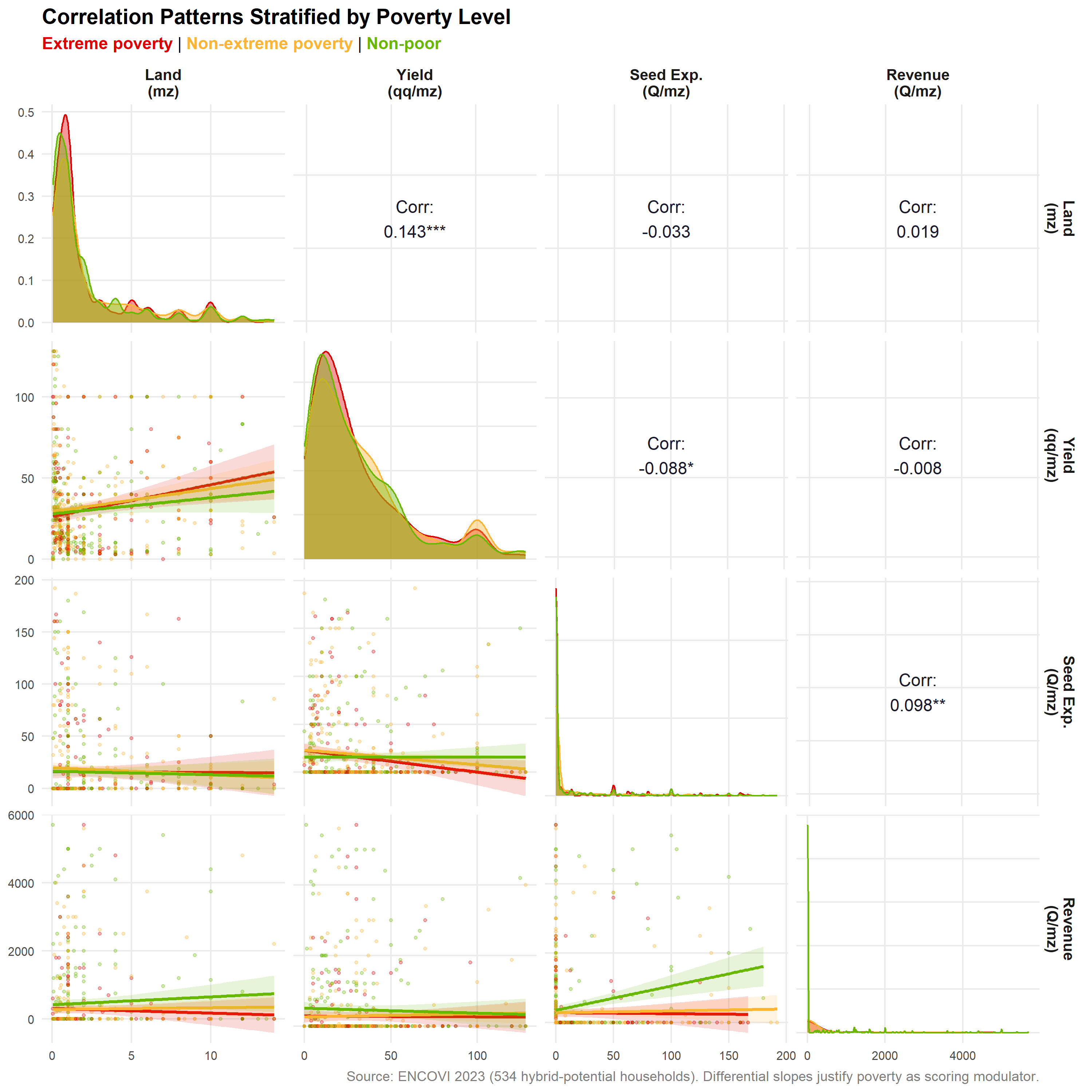
Stratified correlation analysis reveals that poverty status modulates the relationship between agricultural variables. The differential patterns across poverty levels justify including poverty as a scoring modulator.

Pairwise correlation matrix of four variables: land, yield, seed expenditure and revenue. Diagonal cells show density curves, lower cells show scatter plots with linear fits, and upper cells show correlation coefficients, all split by three poverty levels (extreme poverty, non-extreme poverty and non-poor) shown in different colors. The fitted slopes differ across poverty levels, justifying poverty as a scoring modulator. — Figure 6: Correlation patterns stratified by poverty level

Poverty as Modulator

The stratified correlation matrix reveals differential slopes across poverty levels. Farmers in extreme poverty show distinct investment-yield relationships compared to non-poor farmers, justifying the inclusion of poverty level as a scoring modulator.

Stratified Analysis: Land Ownership as Modulator

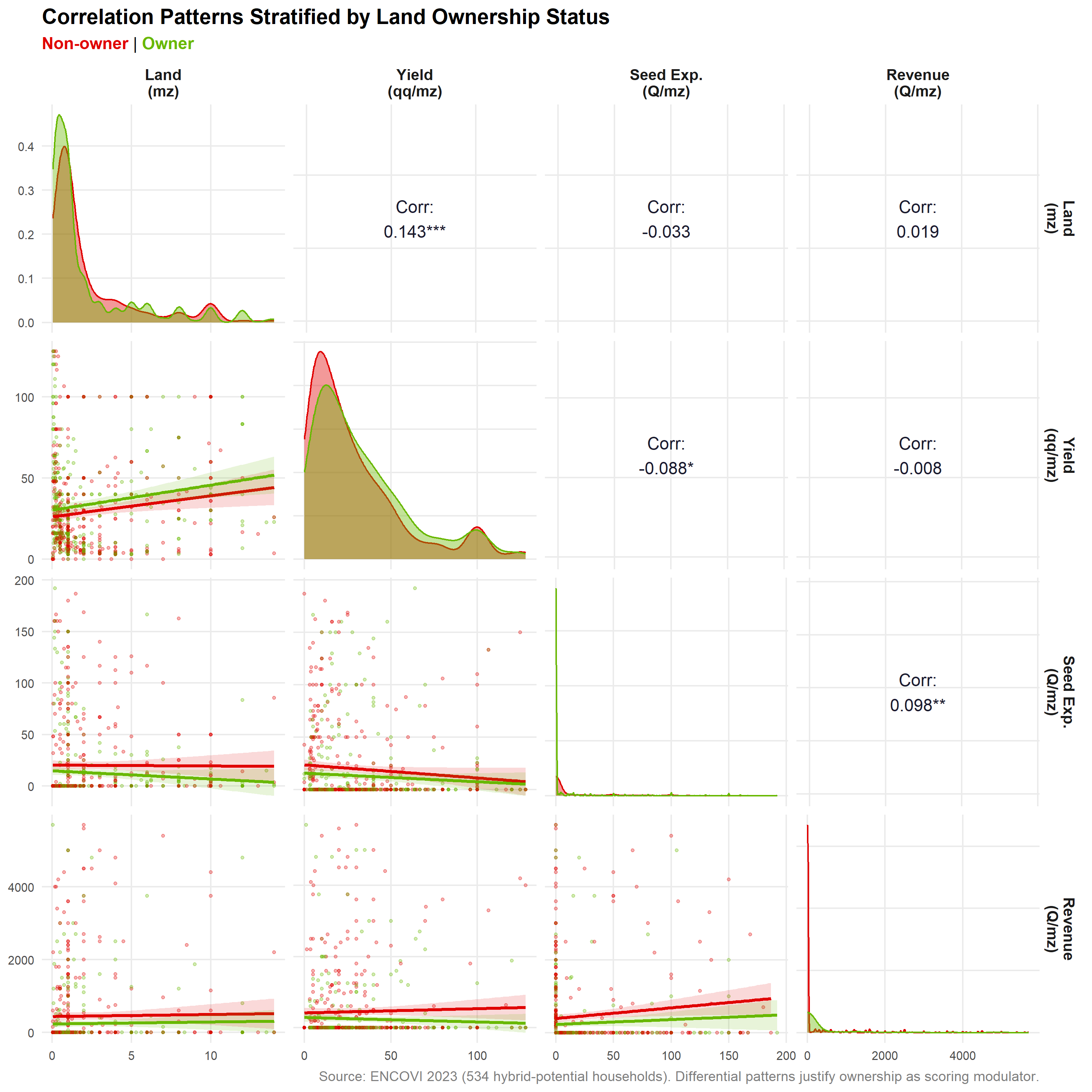
Land ownership status modulates agricultural performance patterns. Owners and non-owners exhibit distinct investment-yield dynamics.

Excluded Variables: Age and Education

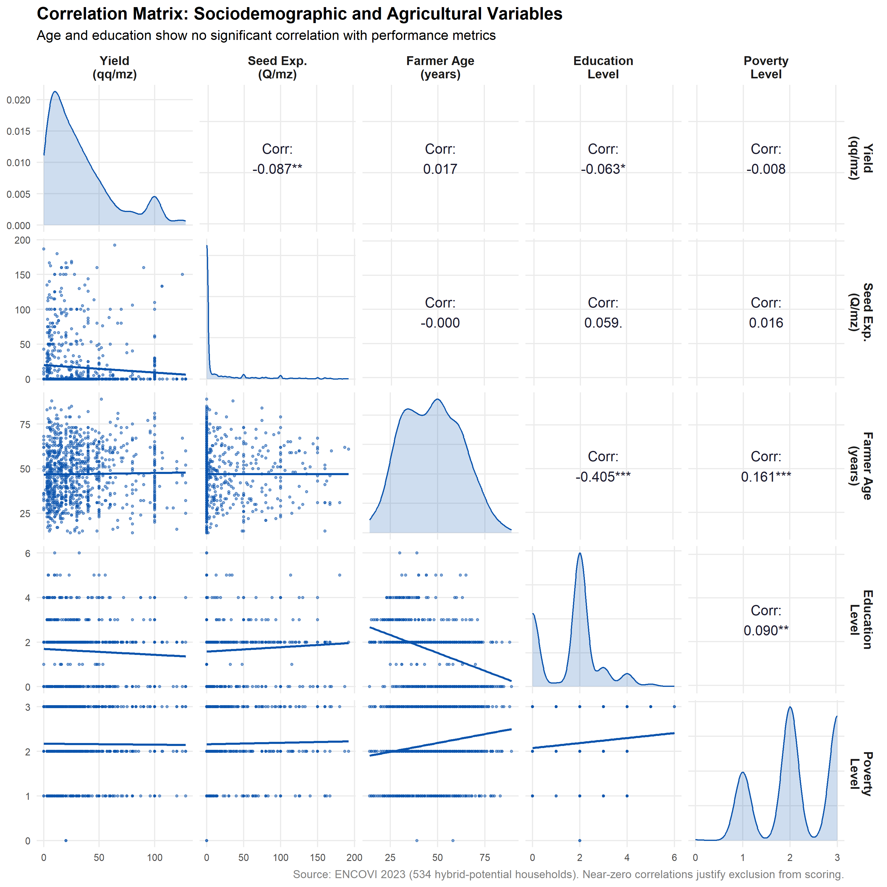
Farmer age and education level were evaluated as potential scoring components. The correlation matrix reveals that these variables show no systematic relationship with agricultural performance metrics, leading to their exclusion from the scoring system.

Pairwise correlation matrix of five variables: yield, seed expenditure, farmer age, education level and poverty level. Diagonal cells show density curves, lower cells show scatter plots with linear fits, and upper cells show correlation coefficients. The coefficients linking farmer age and education to the agricultural performance metrics are near zero, supporting their exclusion from the scoring system. — Figure 8: Correlation matrix of sociodemographic and agricultural variables

Variables Excluded from Scoring

Age and education level show near-zero correlations with yield and seed expenditure. Their inclusion would add noise without improving segmentation accuracy. The scoring system therefore focuses on variables with demonstrated predictive power: yield z-score, seed expenditure z-score, poverty level, and land ownership.

Scoring System Design

The farmer_score ranges from 0 to 100, with higher values indicating greater likelihood of using non-hybrid seed and lower values greater likelihood of commercial hybrid use. The empirical findings from both frameworks and from the correlation analysis lead to a hurdle model structure:

Zero seed expenditure: deterministic score = 100
Positive seed expenditure: continuous score built from weighted components

The four scoring components are:

Seed expenditure z-score (primary): weighted by the LDA importance of seed expenditure on cluster separation, applied with inverse direction, so lower expenditure raises the non-hybrid likelihood.
Yield z-score (primary): weighted by the LDA importance of yield on cluster separation, applied with inverse direction, so lower yield raises the non-hybrid likelihood.
Poverty level (modulator): the stratified correlation analysis shows different slopes by poverty level. Higher poverty raises the non-hybrid likelihood.
Land ownership (modulator): investment-performance dynamics differ between owners and non-owners. Non-ownership raises the non-hybrid likelihood.

Scoring Logic

For primary variables (yield and seed expenditure z-scores), points are assigned using percentile-based rescaling:

\[\text{Score}_{\text{yield}} = (1 - \text{percentile}_{\text{yield}}) \times W_{\text{yield}}\]

\[\text{Score}_{\text{seed}} = (1 - \text{percentile}_{\text{seed}}) \times W_{\text{seed}}\]

Interpretation:

Farmers at the bottom of the z-score distribution receive maximum points, placing them at the non-hybrid end of the scale
Farmers at the top receive minimum points, placing them at the hybrid end

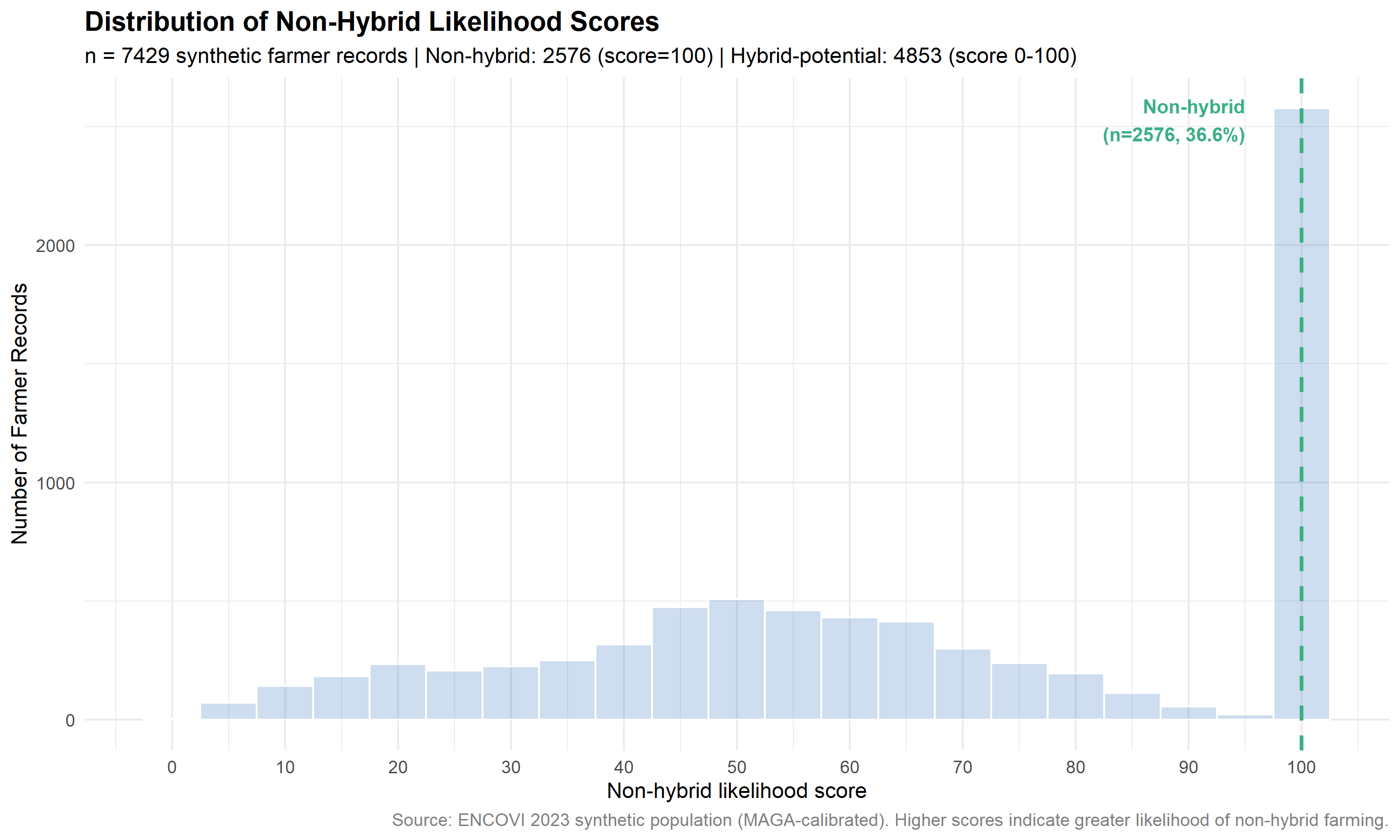
Score Distribution Analysis

Histogram of non-hybrid likelihood scores from 0 to 100 on the x-axis against the number of farmer records on the y-axis. Continuous hybrid-potential scores spread across the range, while a tall spike at a score of 100, marked by a dashed line, captures the non-hybrid farmers who receive the deterministic maximum score for zero seed expenditure. — Figure 9: Distribution of non-hybrid likelihood scores across the synthetic farmer population

Table 6: Score distribution summary by farmer type

Score Distribution Summary. Non-hybrid likelihood scores by farmer type (synthetic population)
Farmer Type	Sample			Score Statistics
Score Distribution Summary
Non-hybrid likelihood scores by farmer type (synthetic population)
Farmer Type	Records	Weighted N	% Population	Min	Max	Mean	Median	SD
OPV-Direct	2576	287,075	36.6%	100	100	100.0	100	0.0
Hybrid-Potential	4853	496,399	63.4%	0	98	49.2	51	20.3
Note: Farmers with zero seed expenditure receive a deterministic score of 100. The rest score between 0 and 100 from their z-scores and modulators.

Threshold Determination

Score thresholds are determined from a target land distribution taken from Semilla Nueva market data on current seed purchasing. Rather than fixing score cutoffs directly, the thresholds are solved so that the share of cultivated land in each segment matches that distribution.

Table 7: Optimal score thresholds for farmer segmentation

Optimal Score Thresholds for Farmer Segmentation. Based on target land distribution (New Seed market data estimates)
Segment	Target Land (mz)	Target %	Cumulative %	Score Threshold
Optimal Score Thresholds for Farmer Segmentation
Based on target land distribution (New Seed market data estimates)
OPV/Criollo	1,437,232	87.0%	87.0%	45
Low	57,200	3.5%	90.5%	40
Mid	76,863	4.7%	95.1%	33
High	80,438	4.9%	100.0%	0
Source: ENCOVI 2023 (MAGA-calibrated). Target distribution from New Seed market data.

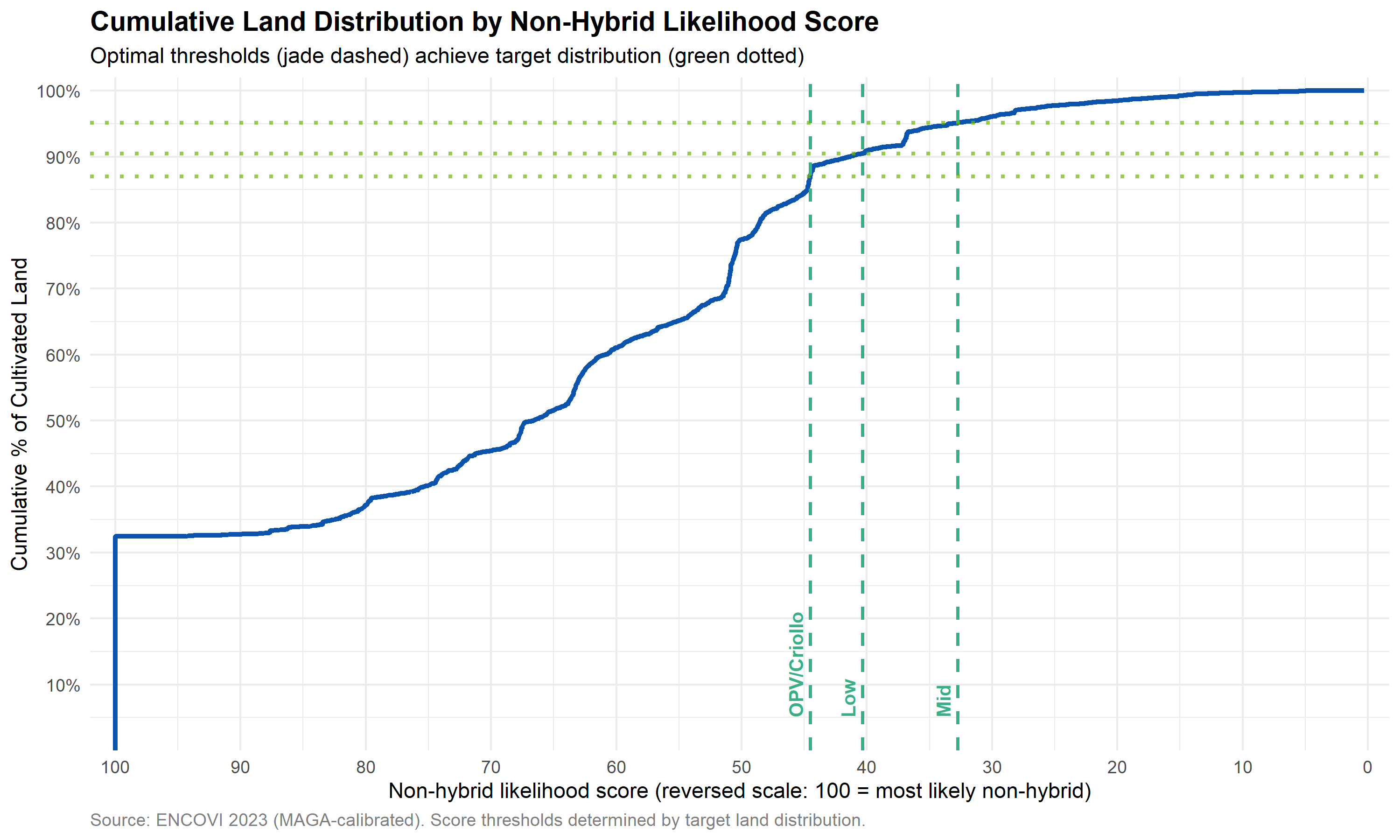
Line chart of the non-hybrid likelihood score on a reversed x-axis, where 100 marks the farmers most likely to use non-hybrid seed, against the cumulative percentage of cultivated land on the y-axis. The curve rises monotonically. Dashed vertical lines mark the optimal score thresholds separating the segments, and dotted horizontal lines mark the target cumulative land shares, showing the thresholds land where the curve meets each target. — Figure 10: Cumulative land distribution by non-hybrid likelihood score with the selected thresholds

Threshold-Based Segmentation

The thresholds are read off the cumulative land distribution curve so that each segment holds its target share of cultivated land, taken from Semilla Nueva’s field estimates of current seed technology adoption. Those targets are heavily concentrated: 87.0% of white maize land sits in the non-hybrid segment, against 3.5%, 4.7% and 4.9% for Low, Mid and High. The resulting cutoffs are 44.5, 40.4 and 32.8 points, so the three purchased-seed segments are separated by a narrow band at the top of the score scale.

Final Segment Characteristics

Table 8: Final segment characteristics (synthetic farmer population)

Final Segment Characteristics. n = 7429 synthetic farmer records
Segment	Distribution			Score Range			Agricultural Profile
Final Segment Characteristics
n = 7429 synthetic farmer records
Segment	Records	% Farmers	% Land	Mean	Min	Max	Yield (qq/mz)	Seed Exp (Q/mz)	Land (mz)
OPV/Criollo	5627	75.9%	87.1%	80.2	45	100	29.7	40	2.4
Low	313	4.1%	3.4%	42.5	40	45	41.4	302	1.7
Mid	411	5.6%	4.7%	36.8	33	40	44.2	525	1.8
High	1078	14.3%	4.8%	20.2	0	33	81.2	1,059	0.7
Source: ENCOVI 2023 (MAGA-calibrated synthetic population). Segments assigned by optimal score thresholds.

Segment Interpretation

OPV/Criollo, the non-hybrid segment: zero or minimal seed expenditure and the lowest yields, the group with most room for a yield increase
Low: some seed investment at below-average intensity
Mid: average seed investment and yields, consistent with mid-level hybrid seed
High: the highest seed investment and yields, consistent with premium hybrid seed already in use

Segmentation Validation

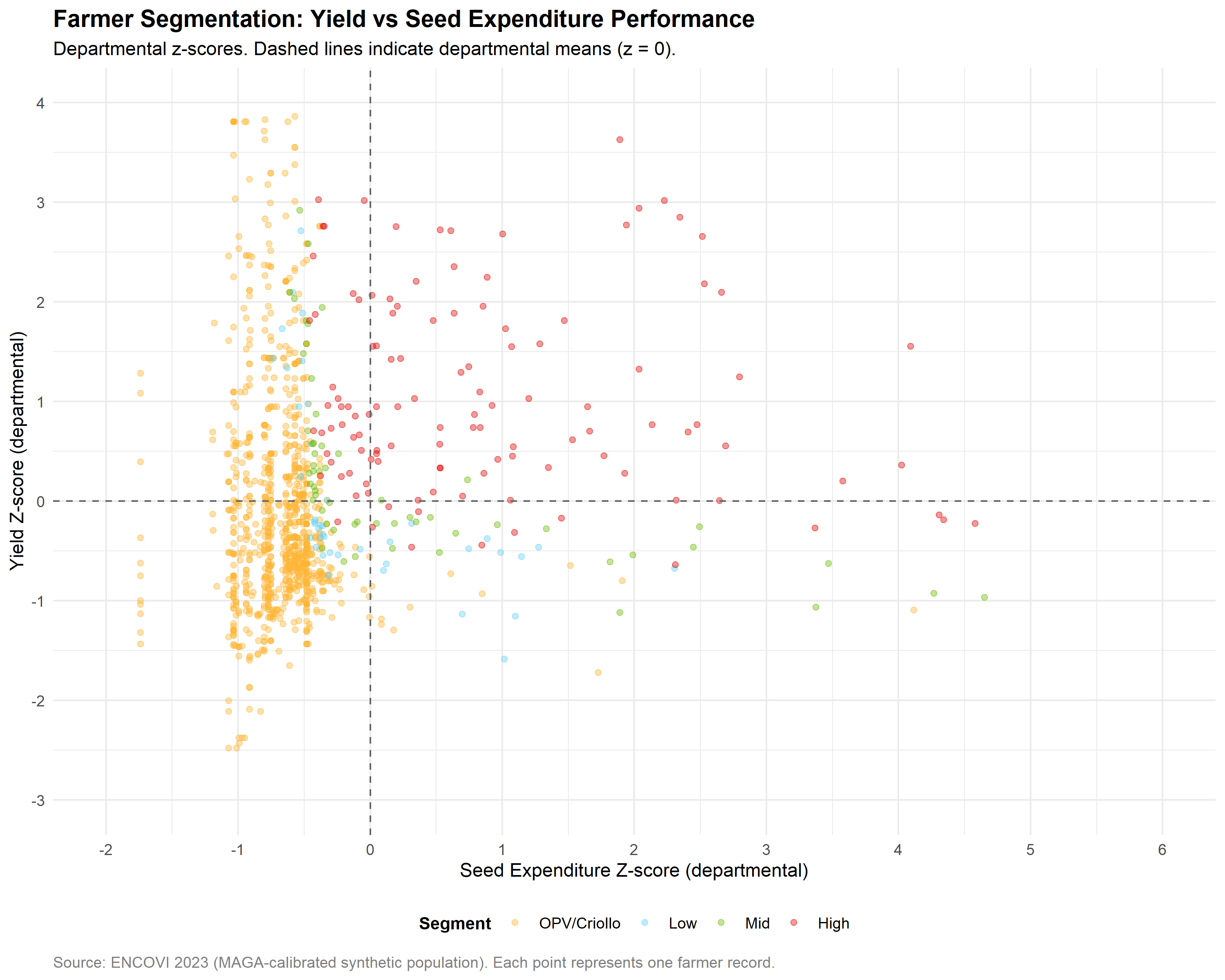
The segment assignment is displayed in the yield × seed expenditure z-score space. Non-hybrid farmers concentrate in the low-expenditure region and high-technology farmers in the high-yield, high-expenditure quadrant.

Scatter chart of seed expenditure z-score on the x-axis against yield z-score on the y-axis, with dashed reference lines at the departmental means (zero) and points colored by final segment (OPV/Criollo, Low, Mid, High). OPV/Criollo points concentrate in the low-expenditure region on the left and High points in the high-yield, high-expenditure upper-right, with Low and Mid in between, confirming that the segments occupy distinct regions of the performance space. — Figure 11: Farmer segmentation in yield-seed expenditure space

Spatial Separation

The segments occupy separate regions of the bidimensional performance space:

OPV/Criollo (orange), the non-hybrid segment: low-expenditure region, on the left
High (red): high-yield, high-expenditure quadrant, upper right
Low and Mid: intermediate positions, with the transition between them gradual rather than sharp

Detailed Segment Profiles

Two complementary summaries characterize the final segments. The first reports survey-weighted medians with interquartile ranges (Q25, Q75), which are robust to outliers and reflect the typical farmer in each segment. The second reports survey-weighted trimmed means (excluding the 5th and 95th percentiles) with standard errors, enabling parametric comparisons across segments while limiting outlier influence.

Survey-Weighted Medians (with IQR)

Table 9: Farmer characteristics by final segment (survey-weighted medians)

Farmer Characteristics by Final Segment. Survey-weighted medians and totals
	OPV/Criollo	Low	Mid	High
Farmer Characteristics by Final Segment
Survey-weighted medians and totals
General
Total Farmers	594,812	32,354	44,169	112,140
% Land	87.1%	3.4%	4.7%	4.8%
% Sellers	21.4%	37.5%	37.4%	41%
Statistics (All Farmers)
Land (mz) [Q25, Q75]	1 [0.48, 2]	0.78 [0.35, 1.09]	0.5 [0.23, 1]	0.29 [0.11, 0.97]
Production (qq) [Q25, Q75]	16 [8, 40]	21 [12, 50]	20 [10, 39]	20 [10, 54]
Yield (qq/mz) [Q25, Q75]	21 [10, 40]	33 [20, 50]	38 [24, 53]	68 [46, 111]
Yield z-score	-0.4	-0.1	0.2	1.4
Seed Exp (Q/mz) [Q25, Q75]	1 [0, 25]	91 [24, 335]	226 [47, 500]	624 [259, 1415]
Seed Exp z-score	-0.6	-0.4	-0.4	0.5
Statistics (Sellers Only)
Revenue (Q) - Sellers	1,700	2,700	2,368	5,934
Gain (Q/qq) - Sellers	109.7	74.8	64.9	70.5
Source: ENCOVI 2023 (MAGA-calibrated). Segments assigned via optimal score thresholds. Values shown as Median [Q25, Q75] where applicable.

Survey-Weighted Trimmed Means (with SE)

Table 10: Farmer characteristics by final segment (survey-weighted trimmed means)

Farmer Characteristics by Final Segment. Survey-weighted TRIMMED MEANS and standard errors (P5-P95)
	OPV/Criollo	Low	Mid	High
Farmer Characteristics by Final Segment
Survey-weighted TRIMMED MEANS and standard errors (P5-P95)
General
Total Farmers	594,812	32,354	44,169	112,140
% Land	87.06%	3.43%	4.71%	4.80%
% Sellers	21.44%	37.53%	37.41%	41.05%
Statistics (All Farmers)
Land (mz) [Mean ± SE]	1.620 (±0.032)	1.068 (±0.077)	1.029 (±0.120)	0.752 (±0.039)
Production (qq) [Mean ± SE]	39.59 (±0.91)	39.17 (±2.88)	30.39 (±1.89)	35.51 (±1.41)
Yield (qq/mz) [Mean ± SE]	29.22 (±0.39)	37.76 (±1.61)	40.92 (±1.24)	63.29 (±1.04)
Yield z-score [Mean ± SE]	-0.115 (±0.015)	0.229 (±0.064)	0.328 (±0.047)	1.271 (±0.039)
Seed Exp (Q/mz) [Mean ± SE]	34.98 (±1.51)	211.48 (±25.20)	276.38 (±17.24)	499.35 (±15.27)
Seed Exp z-score [Mean ± SE]	-0.625 (±0.004)	-0.267 (±0.032)	-0.188 (±0.027)	0.179 (±0.020)
Statistics (Sellers Only)
Revenue (Q) - Sellers [Mean ± SE]	2866.47 (±115.67)	3480.13 (±321.32)	4989.87 (±460.10)	5926.68 (±238.78)
Gain (Q/qq) - Sellers [Mean ± SE]	97.27 (±2.79)	85.49 (±11.71)	56.05 (±10.73)	62.53 (±5.98)
Source: ENCOVI 2023 (MAGA-calibrated). Trimmed means exclude P5 and P95 to reduce outlier influence.

Summary

Methodological Framework

Element	Approach	Rationale
Standardization	Departmental z-scores	Separates regional agro-climatic conditions from technology choice
Segmentation	Dual-framework (PAM + quadrant)	Two independent routes to the same grouping, compared against each other
Scoring	Hurdle model: deterministic zero-expenditure branch + continuous branch	Matches the zero-inflated expenditure distribution
Weights	LDA-derived from cluster separation	Read from the data rather than set by hand
Modulators	Poverty + Land ownership	Stratified correlation analysis shows different slopes
Thresholds	Cumulative land distribution	Reproduces the target land distribution from Semilla Nueva market data

Key Findings

Dual-framework convergence: The two frameworks agree on 78.7% of households, with the closest correspondence at the non-hybrid end (221 of 240 households in PAM cluster 3).
LDA-informed weights: Yield and seed expenditure contribute in near-equal measure to cluster separation.
Stratified modulation: Poverty level and land ownership relate to agricultural performance with different slopes across strata, which is what places them in the scoring as secondary modulators.
Target-based thresholds: The score boundaries reproduce Semilla Nueva’s field estimates of current seed technology adoption, under which 87.0% of white maize land is non-hybrid.

Application

The segmentation enables:

Differential economic parameters by segment for impact calculation
Adoption priority scoring based on segment characteristics
Targeting strategies for biofortification promotion