Prepare Nutrient Transfer Modeling Data

Module 3: Transfer Models

Why Transfer Models?

Children in the SIVESNU 2018 data (the nutrition surveillance system) have anthropometric measurements (height, weight) but no dietary intake data. Meanwhile, ENCOVI 2023 households have detailed food consumption records but no child growth measurements.

Transfer models bridge this gap: we use demographic and socioeconomic characteristics common to both datasets to predict nutrient intake for SIVESNU children based on patterns observed in ENCOVI.

Overview

This document describes the data preparation steps required before building prediction models. High-quality models require:

Complete data — Missing values must be handled appropriately
Independent predictors — Highly correlated variables create instability
Informative variables — Variables with no variation provide no predictive value
Normalized distributions — Extreme skewness can bias predictions

Data Loading and Variable Selection

Source Data

We start with the individual-level nutrient intake dataset created in Module 1, containing the full sample of individuals from ENCOVI 2023 across all 22 departments of Guatemala.

Predictor Variables

Transfer models predict nutrient intake based on characteristics that are available in both ENCOVI and SIVESNU. The shared variables span six categories:

Category	Variables
Demographic	Age, sex, household relationship
Geographic	Department, urban/rural area
Household composition	Number of members, education level, property ownership
Housing characteristics	Dwelling type, construction materials, rooms, sanitation
Basic services	Water source, garbage collection
Household assets	Electricity, television, telephone, computer

Variables unique to one dataset (e.g., detailed food consumption in ENCOVI, anthropometric measurements in SIVESNU) cannot be used as predictors.

Functional Form of the Predictors

The candidate set entering each nutrient model comprises 20 terms, with the functional form set by the type of variable:

Continuous predictors enter as orthogonal polynomials: age at degree 2, and household members, mean household education and number of rooms at degree 3. The polynomial terms let intake vary non-linearly across the range of each variable, which matters for age in particular, where intake rises steeply through childhood and flattens in adulthood.
Nominal predictors (household relationship, sex, department, urban/rural area, property regime, dwelling type, construction materials, sanitation, water source, garbage collection, and the asset indicators) enter as factors, contributing one coefficient per level.

Missing Value Treatment

Why This Matters

Prediction models require complete data for all observations, and the imputation method has to hold the joint structure of the predictors so that later correlation and variance filtering operate on realistic values.

Our Approach: Random Forest Imputation

We use a Random Forest-based multivariate imputation procedure, which predicts missing values based on patterns in the complete data. The implementation uses the missRanger algorithm with a multi-threaded ranger engine for computational efficiency on large surveys. This method:

Preserves correlations between variables
Handles both numeric and categorical data
Provides out-of-bag error metrics (OOBE for continuous, PFC for categorical) to verify imputation accuracy

Missing Data Summary

Table 1: Missing value summary for predictor variables

Missing Values in Predictor Variables. Variables requiring imputation before modeling
Variable	N Missing	% Missing
Missing Values in Predictor Variables
Variables requiring imputation before modeling
recoleccion_basura	2,517	5.47%
tipo_sanitario	2,200	4.78%
cocina	133	0.29%
grado_estudios_hogar	111	0.24%
parentesco	110	0.24%

Only 5 variables have missing data, with the worst case affecting less than 5.5% of observations (recoleccion_basura). Most variables are complete.

Imputation Quality

Table 2: Random Forest imputation quality metrics

Missing Value Imputation Quality Assessment. Out-of-bag error estimates from Random Forest imputation
Metric	Value	Quality Assessment
Missing Value Imputation Quality Assessment
Out-of-bag error estimates from Random Forest imputation
OOBE (Continuous Variables)¹	NA	No continuous variables required imputation
PFC (Categorical Variables)²	0.0875	Acceptable
Number of Iterations	10.0000	Fixed parameter
Trees per Iteration	100.0000	Fixed parameter
¹ OOBE: aggregated out-of-bag error across the continuous variables imputed, bounded in [0, 1] and invariant to their scale. Values < 0.5 indicate acceptable imputation quality for continuous variables.
² PFC: Proportion of Falsely Classified entries. Values < 0.2 indicate acceptable imputation quality for categorical variables.

Quality Assessment

OOBE (for continuous variables) and PFC (for categorical variables) are out-of-bag (OOB) error metrics — calculated from observations that were randomly excluded during tree construction within the Random Forest algorithm, providing an internal quality metric without requiring a separate test set. The ranges conventionally treated as acceptable for this imputation method are OOBE < 0.50 and PFC < 0.20.

OOBE = N/A (no continuous variables required imputation)
PFC = 0.09 (categorical variables) — within the acceptable range

Residual Missing Value Completion

The Random Forest imputation engine can, in rare cases, leave residual missing values for a small subset of rows when the out-of-bag prediction collapses inside a terminal node with zero within-leaf variance. This affects a small fraction of the sample and is resolved by a final completion step, which leaves the predictor matrix complete.

Completion Rule

Residual missing values are completed with a variable-specific rule:

Numeric / integer variables: median of the observed values, which preserves the discrete support of ordinal scales (e.g., years of schooling taking values such as 1, 1.5, 2, 2.5).
Factor variables: mode of the observed values.

Table 3: Residual missing value completion after Random Forest imputation

Residual Missing Value Completion. Values completed by variable-specific rule after RF imputation
Variable	N Completed	Completion Rule
Residual Missing Value Completion
Values completed by variable-specific rule after RF imputation
grado_estudios_hogar	111	Median
— Residual NAs after completion —	0	Integrity check: passed

Integrity Check

The final row of the table reports the number of residual missing values after the completion step. A value of zero means the predictor matrix is complete before correlation analysis, near-zero variance filtering, and model training.

Variable Quality Assessment

Before building models, we evaluate whether all candidate predictors provide useful information. Two common issues can degrade model performance:

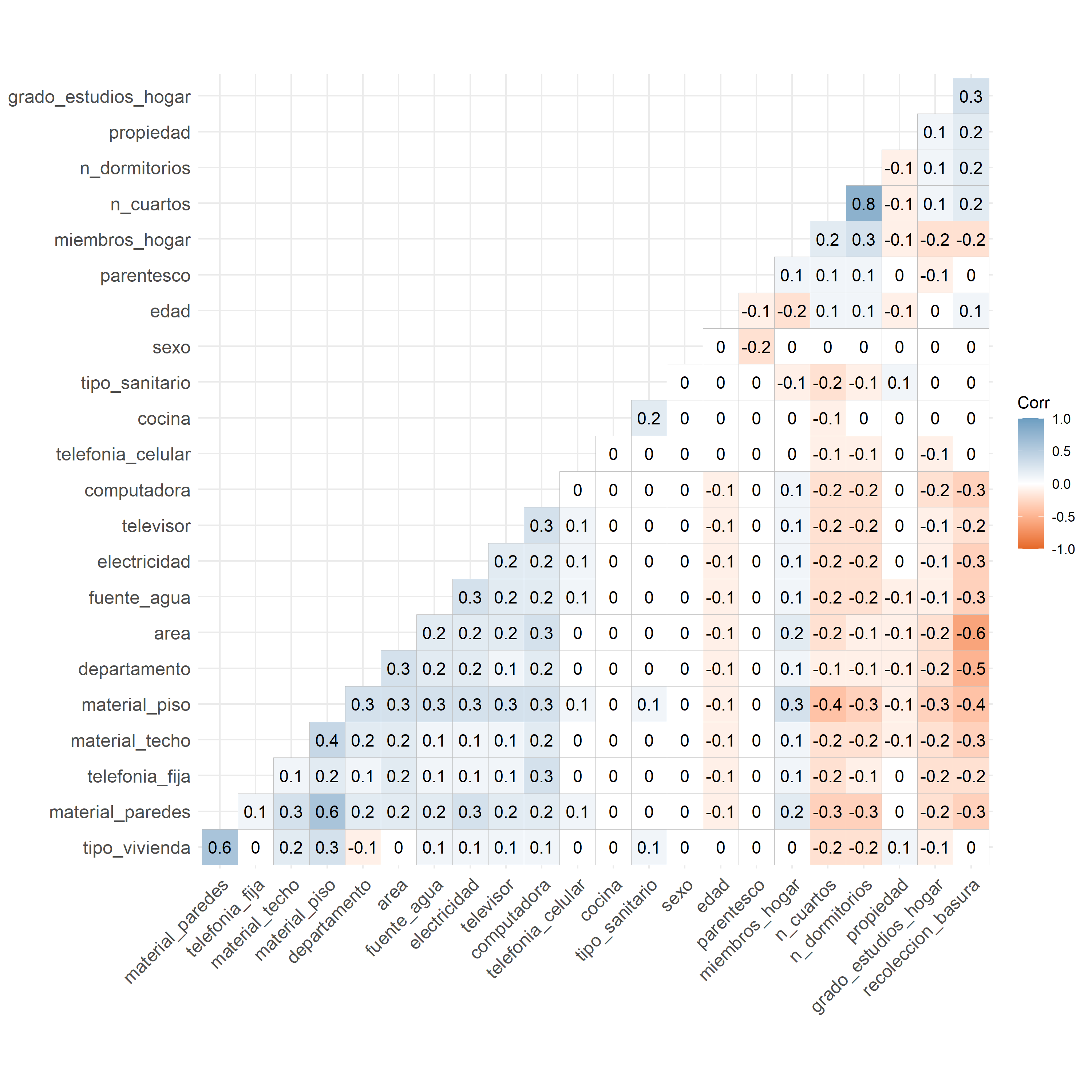
Multicollinearity

When two variables measure essentially the same thing, including both creates redundancy and statistical instability.

Correlation heatmap of the predictor variables, shown as an upper triangular matrix with the same variables along both axes, reordered by hierarchical clustering. Each cell is labelled with its correlation coefficient and colour-coded from orange for negative through white near zero to blue for positive. Most pairs are weakly correlated, but number of bedrooms and total rooms stand out as strongly positively correlated (r = 0.8), flagging the redundancy that leads to dropping one of them. — Figure 1: Correlation matrix of predictor variables

Decision: Remove Redundant Variable

Number of bedrooms (n_dormitorios) correlates strongly (r > 0.8) with total rooms (n_cuartos). Total rooms is retained as the measure of overall dwelling size, and number of bedrooms is dropped from the candidate set.

Near-Zero Variance

Variables where almost all observations fall in a single category provide minimal discriminatory power for prediction.

Table 4: Near-zero variance analysis for predictor variables

Near-Zero Variance Analysis. Predictor variables with potentially insufficient variation
Variable	Frequency Ratio¹	% Unique Values²	NZV Flag³
Near-Zero Variance Analysis
Predictor variables with potentially insufficient variation
parentesco	1.900	2.39%	FALSE
sexo	1.107	0.43%	FALSE
edad	1.039	21.30%	FALSE
departamento	1.179	4.78%	FALSE
area	1.014	0.43%	FALSE
miembros_hogar	1.111	4.13%	FALSE
grado_estudios_hogar	3.857	2.61%	FALSE
propiedad	5.865	1.09%	FALSE
tipo_vivienda	15.767	1.09%	FALSE
material_paredes	3.648	1.96%	FALSE
material_techo	6.065	1.30%	FALSE
material_piso	1.704	1.52%	FALSE
n_cuartos	1.057	2.83%	FALSE
n_dormitorios	1.124	2.17%	FALSE
cocina	76.470	0.43%	TRUE
tipo_sanitario	12.631	0.43%	FALSE
fuente_agua	4.041	1.74%	FALSE
recoleccion_basura	2.989	0.87%	FALSE
electricidad	6.296	0.43%	FALSE
televisor	1.399	0.43%	FALSE
telefonia_fija	37.997	0.43%	TRUE
telefonia_celular	3.043	0.43%	FALSE
computadora	4.842	0.43%	FALSE
¹ Frequency Ratio: ratio of most common to second most common value. Values >19 combined with low uniqueness trigger NZV flag.
² % Unique Values: percentage of unique values relative to total observations. Values <10% combined with high frequency ratio trigger NZV flag.
³ NZV Flag: TRUE indicates near-zero variance. Both freqRatio >19 AND percentUnique <10% must be met.

Decision: Remove Low-Information Variables

Two variables flagged for near-zero variance:

Kitchen type (cocina): nearly all households have the same type
Landline telephone (telefonia_fija): nearly all households lack landlines

These variables cannot meaningfully distinguish between nutrient profiles and are excluded from the model.

Variable Transformations

Why Transform?

Many statistical models assume predictor variables follow approximately normal distributions. Highly skewed variables (e.g., household size, where most households are small but some are very large) can bias predictions.

Yeo-Johnson Transformation

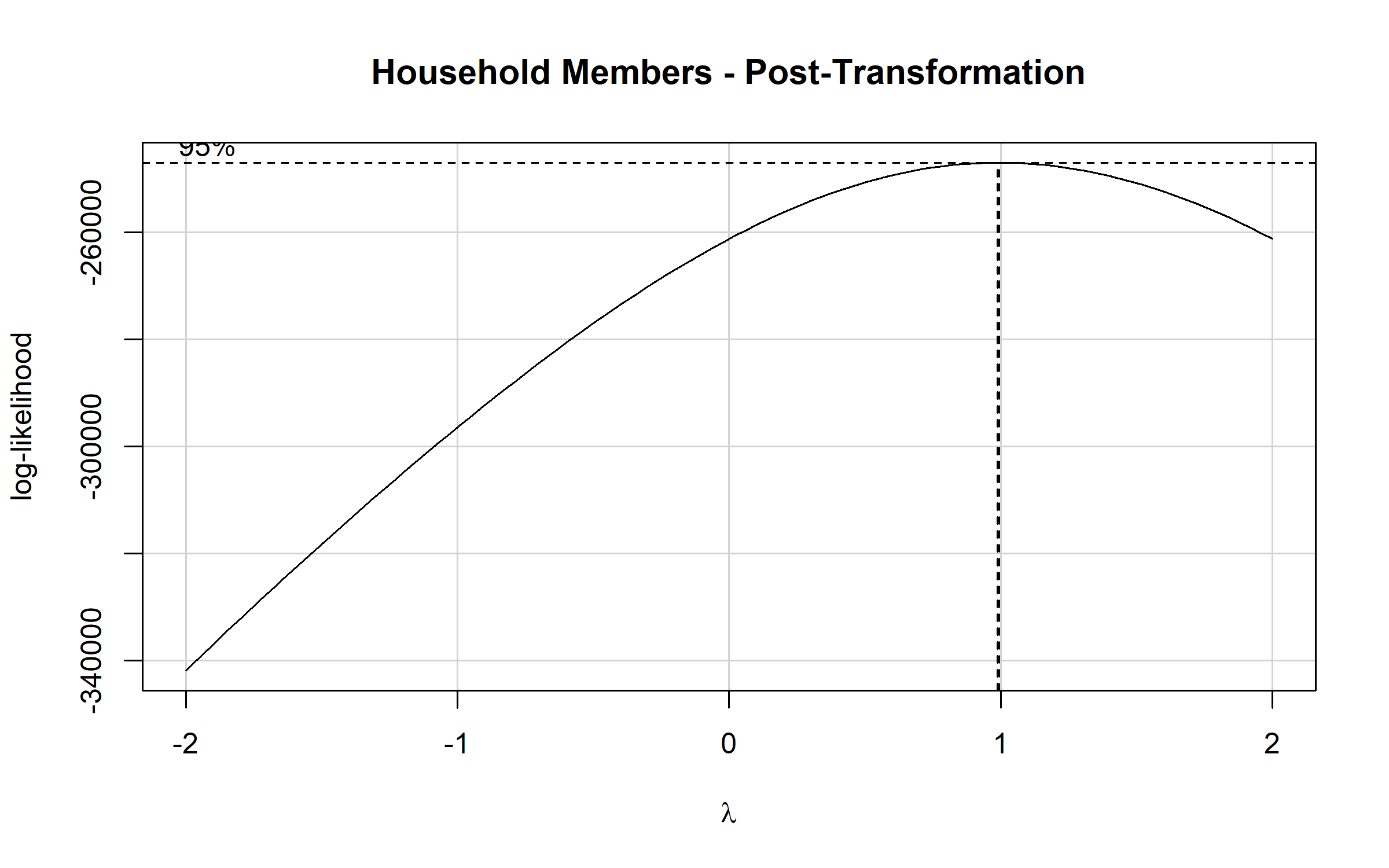
We apply the Yeo-Johnson transformation, which automatically determines the optimal adjustment for each variable. A lambda (λ) value near 1 indicates the variable is already approximately normal; values near 0 indicate logarithmic transformation is needed.

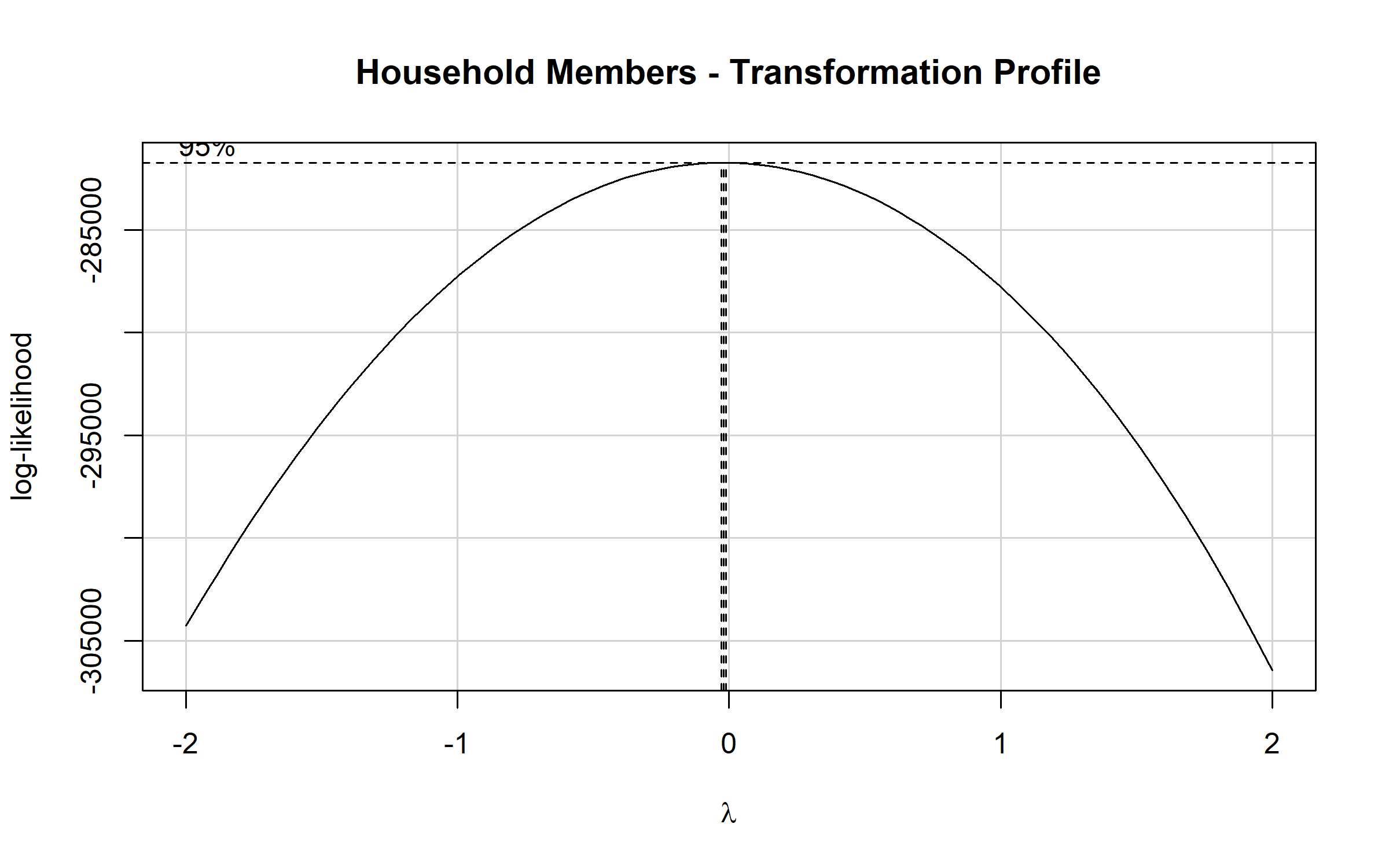
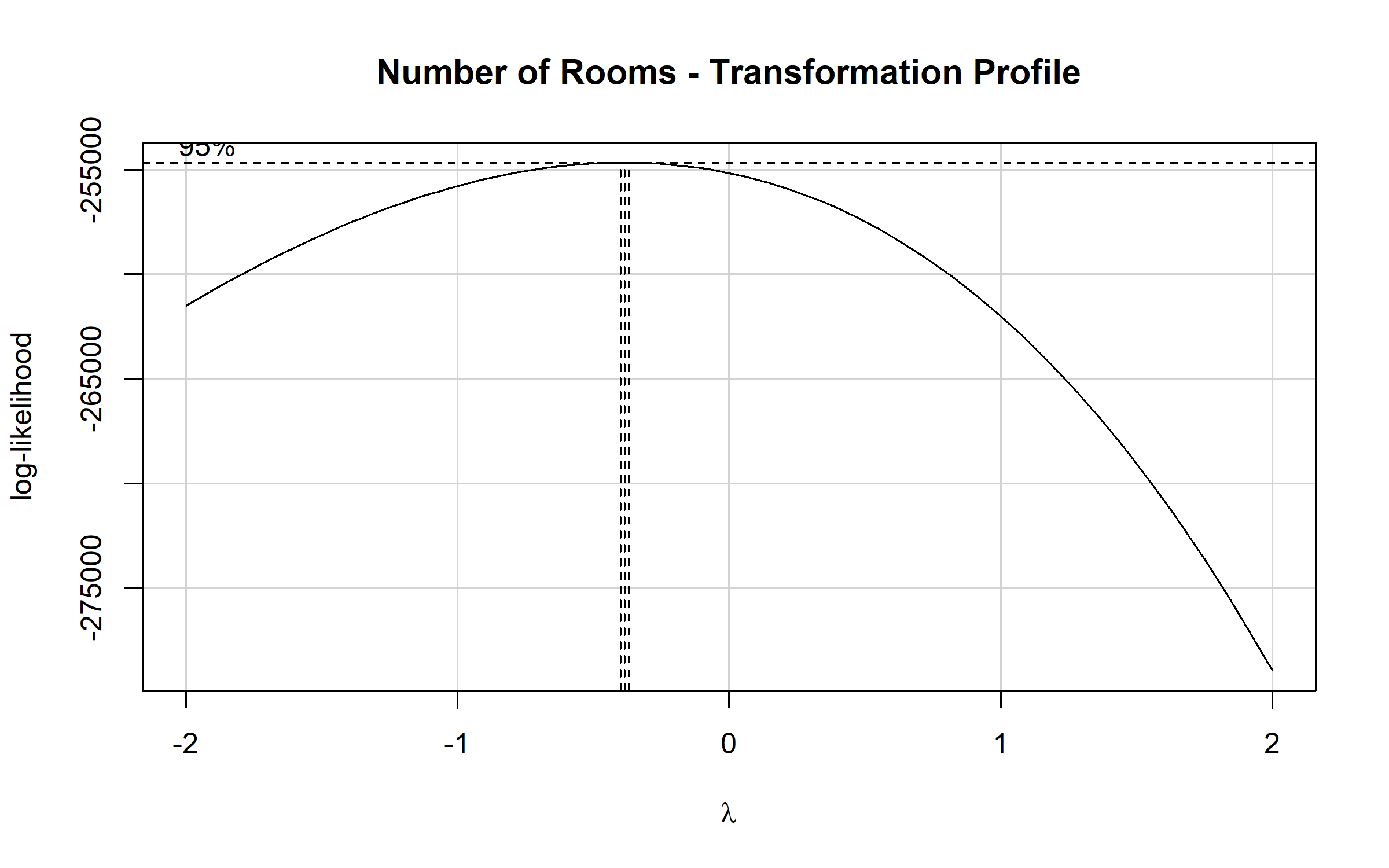
Figure 2: Yeo-Johnson transformation profile for household members

Figure 3: Yeo-Johnson transformation profile for number of rooms

Both household members and number of rooms show λ ≈ 0, indicating right-skewed distributions that benefit from transformation.

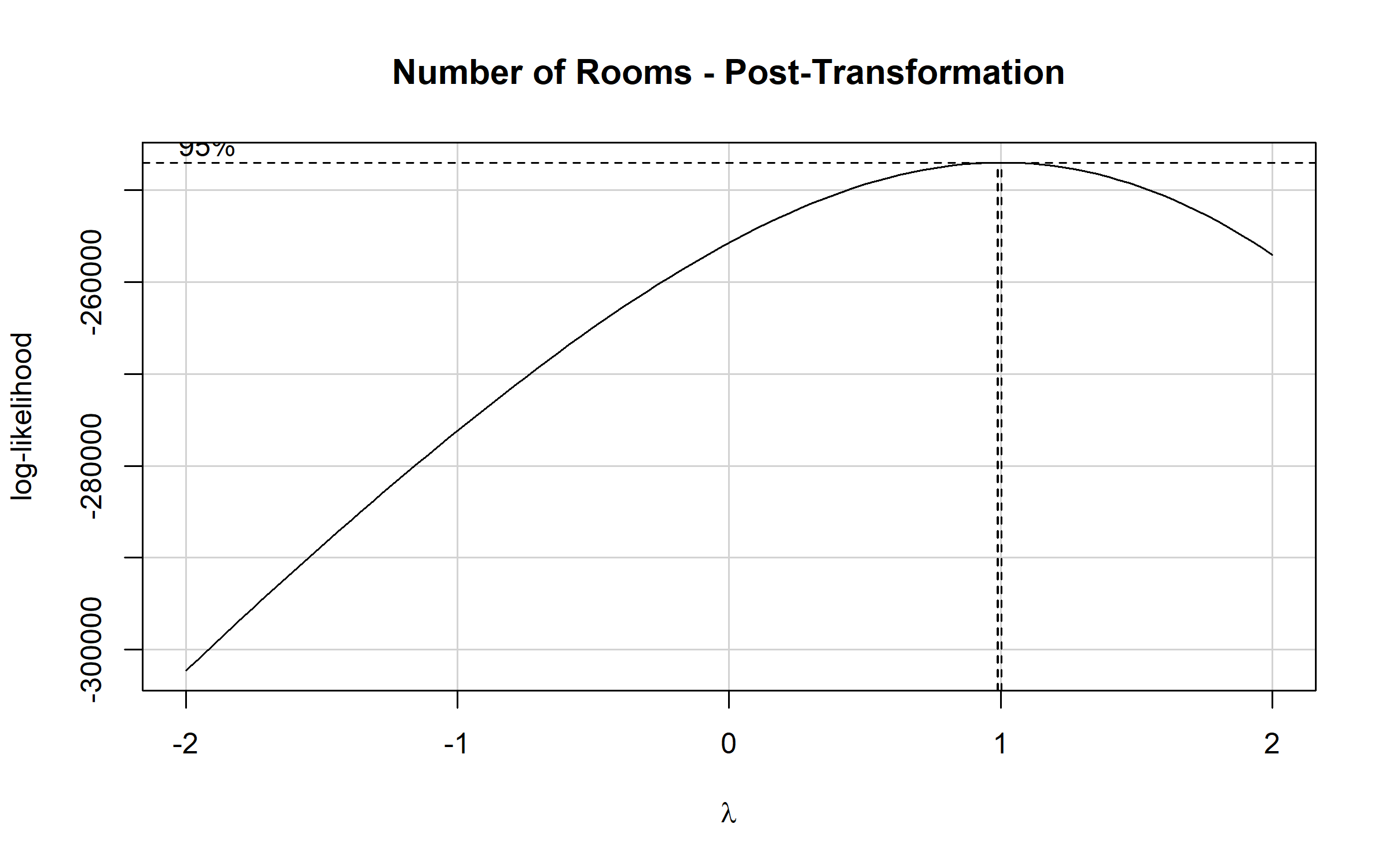
Figure 4: Transformation profile for household members (post-transformation)

Figure 5: Transformation profile for number of rooms (post-transformation)

Transformation Result

After transformation, both variables show λ ≈ 1, the value expected for an approximately normal distribution. The transformation parameters are saved for consistent application to SIVESNU data.

Summary of Data Preparation

This preparation module brings the modeling dataset to the state the transfer models operate on:

Step	Action	Result
Missing values	Random Forest imputation (`missRanger` / `ranger`)	Imputed predictor matrix with OOB diagnostics
Residual completion	Median (numeric) / mode (factor) safety net	100% complete data
Multicollinearity	Remove `n_dormitorios`	Independent predictors
Near-zero variance	Remove `cocina`, `telefonia_fija`	Informative variables only
Normalization	Yeo-Johnson transformation	Improved distributions

Final ENCOVI Dataset

The prepared dataset retains the full sample of individuals from ENCOVI 2023, with predictor variables filtered for quality and continuous predictors normalized via Yeo-Johnson transformation. The transformation parameters are exported for consistent application to SIVESNU data during the modeling of individual nutrients documented in subsequent sections.