| Input Data Summary | |
| SIVESNU 2018 modeling-ready dataset | |
| Item | Value |
|---|---|
| Observations | 773 |
| Boruta-selected predictors | 15 |
| Outcome variable | talla_cm |
| Age range (months) | 6.2 - 59.0 |
| Height range (cm) | 60.6 - 112 |
| Stunting prevalence (HAZ < -2) | 42.2% |
Height Transfer Model
Module 5: Meta-analysis
Why a Height Transfer Model?
The Meta-analysis (Gunaratna) pathway requires predicted height for ENCOVI 2023 children to calculate individual-level impacts of biofortified maize on stunting. Since ENCOVI does not include anthropometric measurements, we train a predictive model on SIVESNU 2018 — which contains direct height data — and apply it across surveys using the shared set of socioeconomic predictors identified when preparing the SIVESNU height data.
We use a Generalized Additive Model (GAM) because the age-height relationship in children under 5 is inherently non-linear: growth velocity is highest in infancy and decelerates progressively. GAMs capture this curvilinear growth trajectory through smooth terms while retaining parametric estimation for categorical predictors. The Gaussian family is appropriate because height conditional on age and covariates is approximately normally distributed.
Input Data
The modeling-ready dataset from the previous step contains 773 SIVESNU 2018 children aged 6-59 months with 15 Boruta-selected predictors and the outcome variable (talla_cm).
GAM Specification
Each predictor receives a model term appropriate to its data type. Continuous predictors with expected non-linear effects use smooth terms (s()), while binary and unordered categorical predictors enter as parametric (linear) terms. Department enters through a penalized random-effect term, which lets the estimation shrink the geographic contribution according to the support the data provide for it.
| Predictor Variables and GAM Specification | |||
| 15 Boruta-selected predictors with assigned model terms | |||
| Variable | R Class | Unique Values | GAM Term1 |
|---|---|---|---|
| edad | numeric | 615 | s(edad, k = 10) |
| area | factor | 2 | parametric: area |
| recoleccion_basura | factor | 4 | parametric: recoleccion_basura |
| departamento | factor | 22 | s(departamento, bs = 're') |
| fuente_agua | factor | 8 | parametric: fuente_agua |
| material_piso | factor | 6 | parametric: material_piso |
| televisor | factor | 2 | parametric: televisor |
| grado_estudios_hogar | numeric | 10 | s(grado_estudios_hogar, k = 5) |
| material_paredes | factor | 8 | parametric: material_paredes |
| telefonia_celular | factor | 2 | parametric: telefonia_celular |
| electricidad | factor | 2 | parametric: electricidad |
| propiedad | factor | 5 | parametric: propiedad |
| computadora | factor | 2 | parametric: computadora |
| tipo_sanitario | factor | 2 | parametric: tipo_sanitario |
| sexo | factor | 2 | parametric: sexo |
| 1 Blue rows: smooth (non-linear) terms. White rows: parametric (linear) terms. | |||
Outcome Distribution
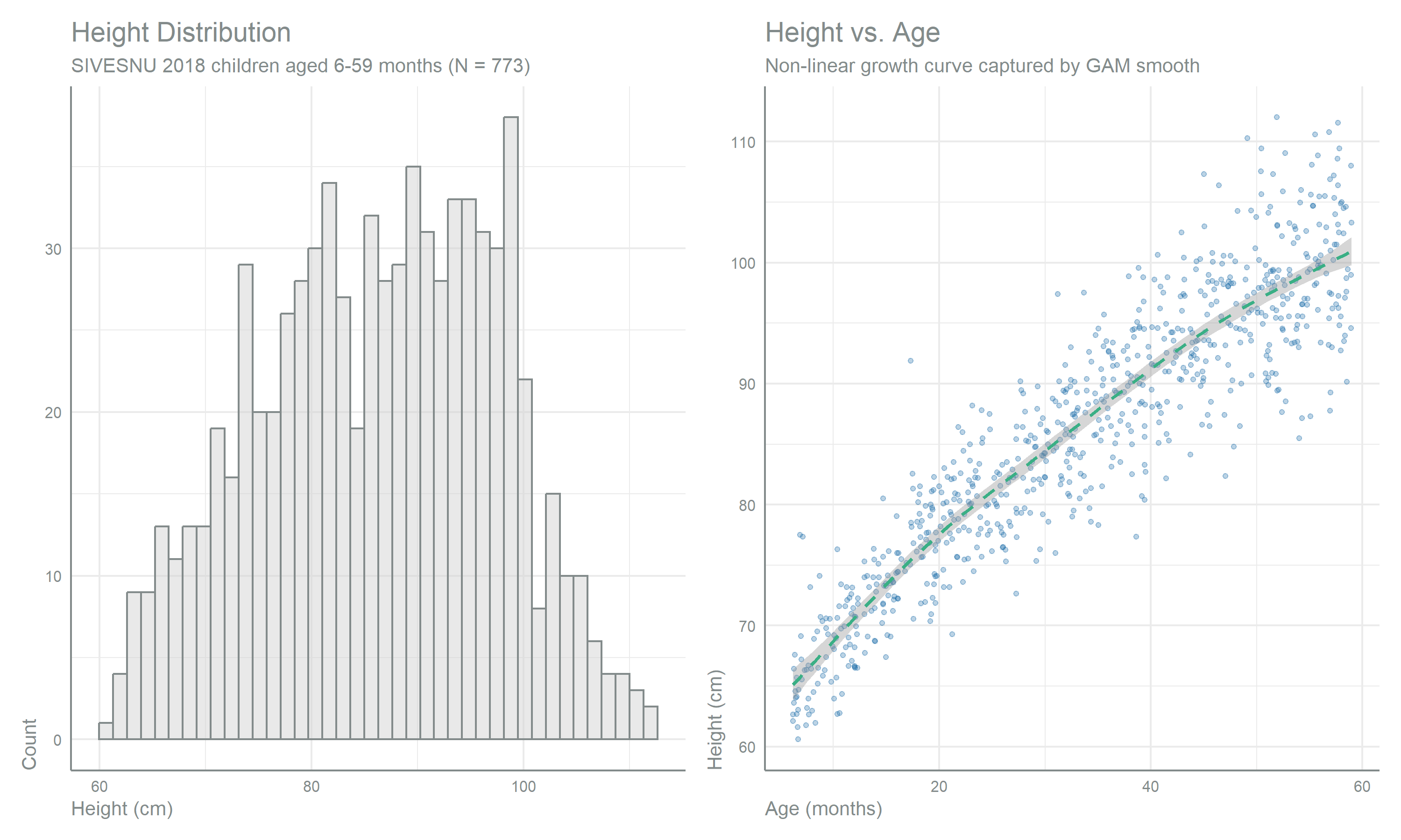
The height distribution spans 60.6 - 112 cm with a slight left skew, consistent with a stunting prevalence of 42.2% in this population. The age-height scatterplot shows the non-linear growth trajectory, with rapid gains in the first two years easing into a more gradual increase after 24 months, which is the pattern the GAM smooth terms are specified to capture.
GAM Model Training
The training pipeline first expands the SIVESNU dataset by survey weights (pesonino) to incorporate the sampling design, then collapses rare factor levels (n < 10) into existing categories to prevent empty-level issues in cross-validation folds. Ordered factors are converted to numeric for smooth term estimation, and an age group variable is added for stratified cross-validation.
| Modeling Data Summary | |
| After type preparation for mgcv | |
| Metric | Value |
|---|---|
| Original observations (pre-uncount) | 773 |
| Expanded observations (post-uncount) | 1041 |
| Total columns | 20 |
| Predictor variables | 15 |
| Complete cases | 1041 |
The model is then trained with REML (Restricted Maximum Likelihood) smooth parameter estimation.
Smooth Term Significance
The approximate F-tests are significant for all three smooth terms. The effective degrees of freedom (EDF) reported alongside them say how much curvature each one takes up.
| Smooth Term Significance | |||||
| Approximate F-tests for non-linear effects | |||||
| Smooth Term | EDF1 | Ref. df | F | p-value | |
|---|---|---|---|---|---|
| s(edad) | 4.25 | 5.23 | 1,442.45 | < 0.001 | * |
| s(grado_estudios_hogar) | 2.01 | 2.48 | 5.99 | 0.0014 | * |
| s(departamento_num) | 0.98 | 1.00 | 44.81 | < 0.001 | * |
| 1 EDF = effective degrees of freedom. EDF close to 1 indicates near-linear relationship. | |||||
Note 1: Smooth Term Interpretation
The age smooth takes 4.24 effective degrees of freedom, which is the non-linear growth curve. The grado_estudios_hogar smooth takes 2.01, a mild curvature in the education-height relationship. This variable encodes the household’s parental educational attainment as the mean of the head of household and their spouse or partner on a six-point ordinal scale mapped to numeric values (1 = Ninguno/Desconocido, 2 = Solo sabe leer, 4 = Primaria, 7 = Secundaria, 10 = Superior/universitaria). The mean over the conjugal unit is the summary used, and other household members do not enter it. The department term takes 0.98 of its single available degree of freedom, so the penalty leaves it close to unshrunk.
Parametric Coefficients
| Parametric Term Coefficients | |||||
| Linear effects of categorical predictors | |||||
| Term | Estimate | SE | t | p-value | |
|---|---|---|---|---|---|
| (Intercept) | 87.107 | 0.656 | 132.808 | < 0.001 | * |
| areaRural | −0.868 | 0.389 | −2.228 | 0.0261 | * |
| sexoMujer | −1.282 | 0.235 | −5.445 | < 0.001 | * |
| recoleccion_basuraServicio privado | 0.155 | 0.458 | 0.338 | 0.7351 | |
| recoleccion_basuraLa queman o la entierran | −1.075 | 0.465 | −2.312 | 0.021 | * |
| recoleccion_basuraLa tiran en cualquier lugar | −1.516 | 0.709 | −2.137 | 0.0328 | * |
| fuente_aguaTubería fuera de la vivienda | −0.312 | 0.684 | −0.457 | 0.6481 | |
| fuente_aguaChorro publico | −0.970 | 0.708 | −1.370 | 0.1711 | |
| fuente_aguaPozo perforado | 0.365 | 0.390 | 0.934 | 0.3504 | |
| fuente_aguaRío, lago, manantial | −0.157 | 0.523 | −0.301 | 0.7633 | |
| fuente_aguaAgua de lluvia | 1.165 | 0.909 | 1.281 | 0.2004 | |
| fuente_aguaOtro | 1.517 | 0.341 | 4.442 | < 0.001 | * |
| material_pisoLadrillo de cemento | 0.478 | 0.530 | 0.901 | 0.3676 | |
| material_pisoTorta de cemento | −0.770 | 0.396 | −1.946 | 0.0519 | |
| material_pisoTierra | −1.275 | 0.511 | −2.496 | 0.0127 | * |
| material_pisoOtro | −3.699 | 1.427 | −2.593 | 0.0097 | * |
| televisorNo | −1.390 | 0.323 | −4.308 | < 0.001 | * |
| material_paredesAdobe | 0.049 | 0.384 | 0.127 | 0.8988 | |
| material_paredesMadera | 1.240 | 0.420 | 2.951 | 0.0032 | * |
| material_paredesLamina metalica | 0.434 | 0.554 | 0.783 | 0.4336 | |
| material_paredesBajareque | 2.407 | 1.114 | 2.161 | 0.0309 | * |
| material_paredesLepa, palo o caña | 0.825 | 0.917 | 0.900 | 0.3682 | |
| material_paredesOtro | 0.064 | 0.897 | 0.071 | 0.943 | |
| telefonia_celularNo | −1.315 | 0.395 | −3.330 | < 0.001 | * |
| electricidadNo | −0.205 | 0.410 | −0.500 | 0.6173 | |
| computadoraNo | −0.267 | 0.440 | −0.607 | 0.5439 | |
| propiedadAlquilada | 0.295 | 0.427 | 0.690 | 0.4901 | |
| propiedadCedida o prestada | 0.542 | 0.356 | 1.522 | 0.1284 | |
| propiedadOtro | 1.074 | 1.347 | 0.797 | 0.4255 | |
Overall Model Fit
| Overall Model Fit | |
| GAM with Gaussian family and REML estimation | |
| Metric | Value |
|---|---|
| Deviance explained | 89.3% |
| Adjusted R-squared | 0.8894 |
| GCV score | 2840.43 |
| REML score | 14.02 |
| Scale estimate (residual variance) | 14.02 |
| N observations | 1041 |
NoteModel Fit
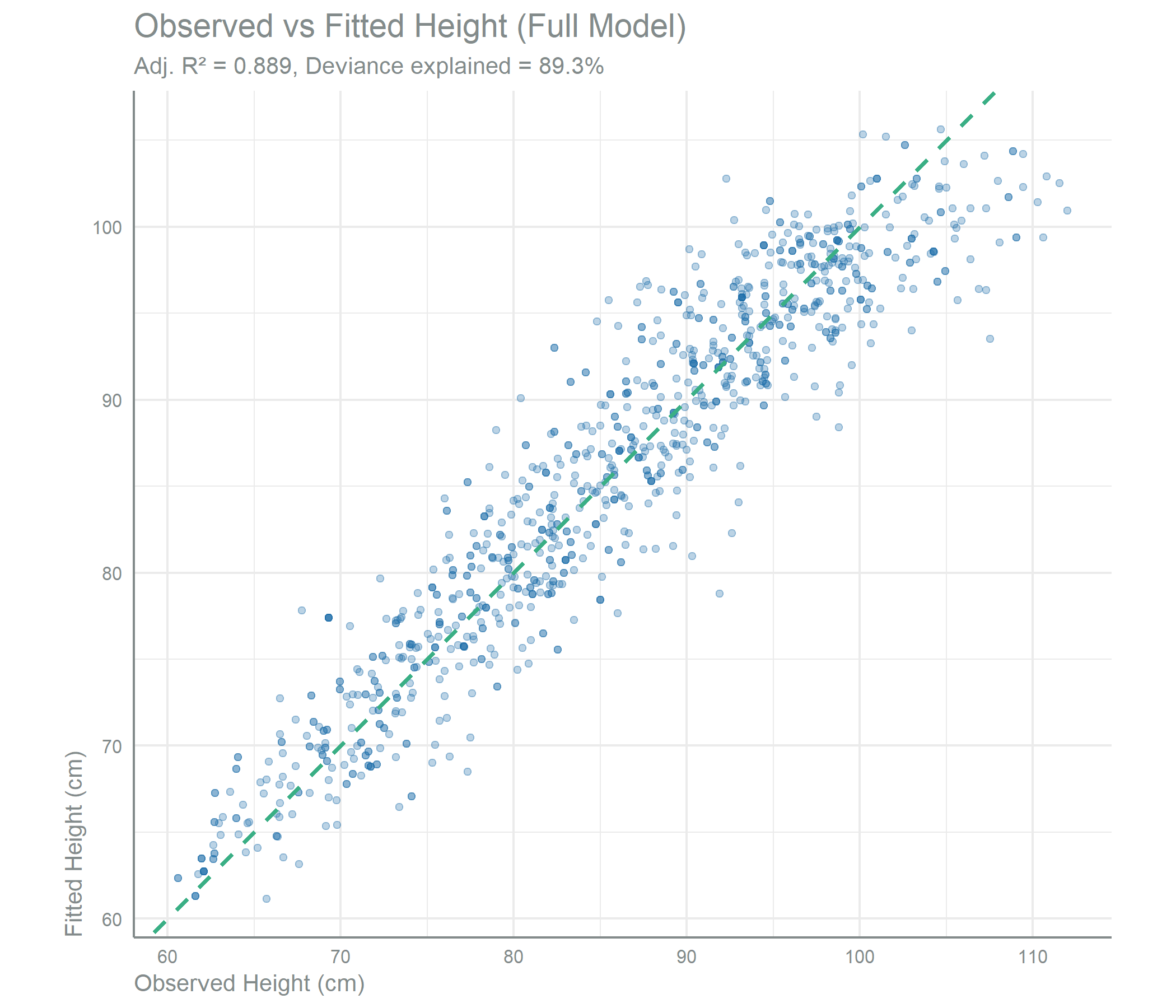
The GAM accounts for 89.3% of deviance (Adj. R² = 0.889) on the training data. Age carries most of this, as expected for child height. Beyond it, the parametric block contributes significant coefficients for child sex, water source, television ownership, mobile phone access, area of residence, floor and wall materials, and refuse collection.
Cross-Validation
10-Fold Stratified CV
We evaluate out-of-sample prediction performance using stratified 10-fold cross-validation. Stratification by age group gives each fold a representative spread along the growth curve.
| Cross-Validation Performance Summary | |
| 10-fold stratified CV (stratified by age group) | |
| Metric | Value |
|---|---|
| Root Mean Squared Error (cm) | 3.851 |
| Mean Absolute Error (cm) | 3.001 |
| R-squared (out-of-sample) | 0.883 |
| Mean Bias (cm) | -0.013 |
| SD of Residuals (cm) | 3.853 |
| Predictions within +/- 5 cm (%) | 83.093 |
| Predictions within +/- 3 cm (%) | 58.405 |
| Performance by Cross-Validation Fold | |||||
| Stability assessment across folds | |||||
| Fold | N | RMSE (cm) | MAE (cm) | R² | Bias (cm) |
|---|---|---|---|---|---|
| 1 | 106 | 3.81 | 3.02 | 0.886 | −0.13 |
| 2 | 106 | 3.71 | 2.84 | 0.892 | 0.07 |
| 3 | 106 | 3.60 | 2.79 | 0.906 | −0.07 |
| 4 | 105 | 3.57 | 2.77 | 0.901 | 0.00 |
| 5 | 105 | 3.76 | 2.92 | 0.891 | −0.73 |
| 6 | 104 | 4.07 | 3.30 | 0.849 | 0.29 |
| 7 | 103 | 3.76 | 2.90 | 0.889 | 0.26 |
| 8 | 102 | 4.82 | 3.68 | 0.830 | 0.28 |
| 9 | 102 | 3.55 | 2.77 | 0.901 | 0.00 |
| 10 | 102 | 3.72 | 3.04 | 0.877 | −0.09 |
NoteCross-Validation Results
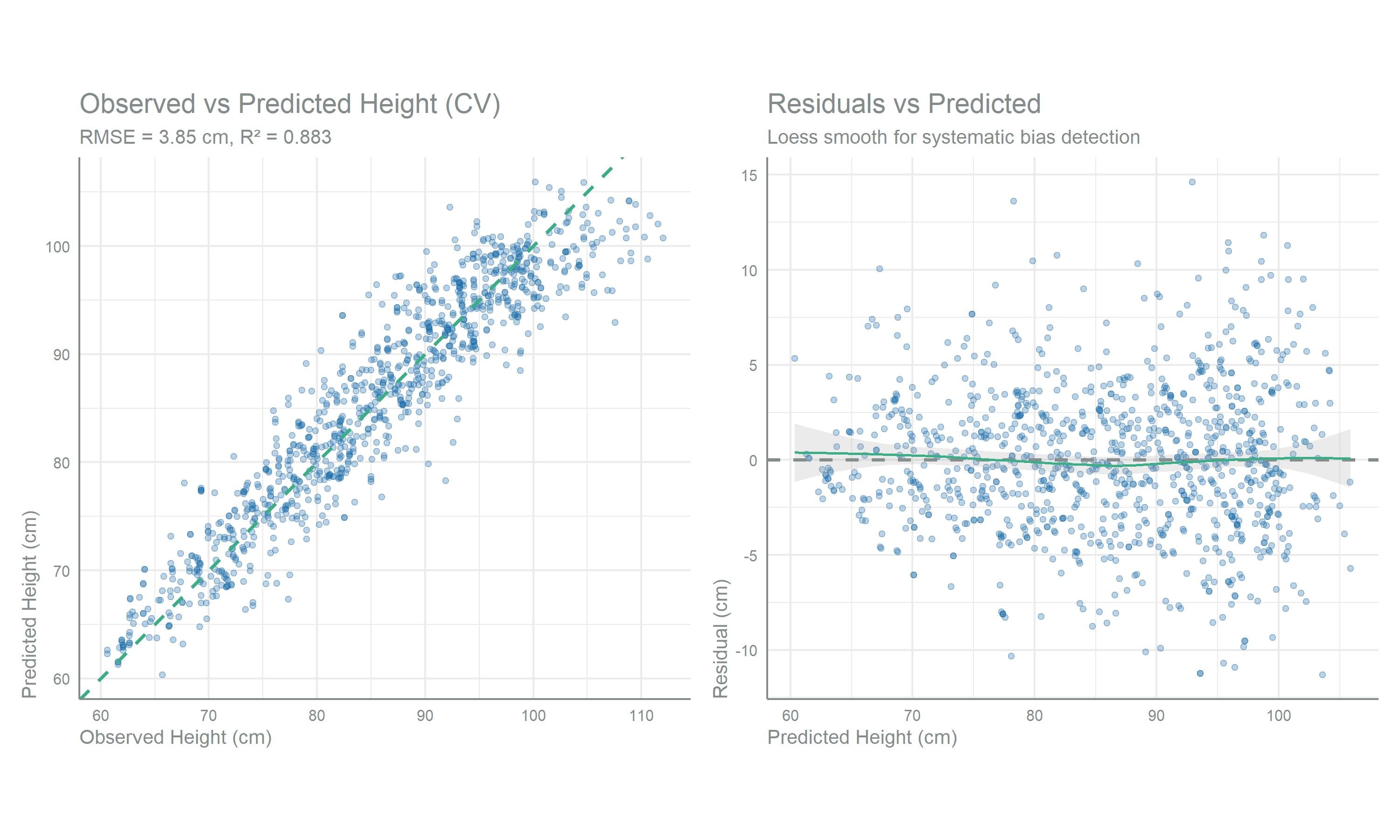
Out-of-sample performance stays close to the in-sample fit: RMSE = 3.85 cm, R² = 0.883, with a mean bias of -0.01 cm. Across the ten folds RMSE ranges from 3.55 to 4.82 cm and R² from 0.83 to 0.906, so the fit does not hinge on which subset is held out. 83.1% of predictions fall within ±5 cm and 58.4% within ±3 cm of observed height.
CV Diagnostic Plots
Performance by Subgroup
By Age Group
| Prediction Performance by Age Group | |||||||
| 10-fold CV results stratified by age | |||||||
| Age Group | N | Mean Height (cm) | RMSE (cm) | MAE (cm) | R² | Bias (cm) | Within ±3 cm (%) |
|---|---|---|---|---|---|---|---|
| 6-11m | 86 | 66.39 | 3.25 | 2.49 | 0.335 | −0.06 | 70.9 |
| 12-23m | 227 | 75.36 | 3.37 | 2.66 | 0.493 | 0.10 | 63.9 |
| 24-35m | 223 | 83.35 | 3.48 | 2.73 | 0.393 | −0.18 | 60.1 |
| 36-47m | 240 | 91.57 | 3.78 | 2.99 | 0.487 | 0.19 | 57.1 |
| 48-59m | 265 | 98.04 | 4.69 | 3.70 | 0.284 | −0.14 | 49.4 |
NoteAge-Dependent Accuracy
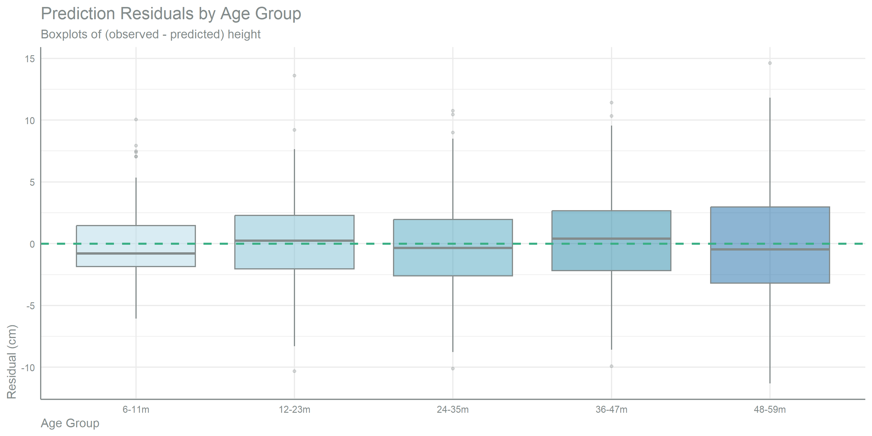
RMSE rises from 3.25 cm in the 6-11 month group to 4.69 cm in the 48-59 month group, as shown in Table 9, which follows the wider spread of height at older ages. Within-group R² values sit between 0.28 and 0.49 because age, the leading predictor, varies little inside each group, leaving the socioeconomic variables and child sex to account for the rest.
By Department
| Prediction Performance by Department | ||||
| 10-fold CV results by geographic unit | ||||
| Department | N | RMSE (cm)1 | MAE (cm) | Bias (cm) |
|---|---|---|---|---|
| Guatemala | 188 | 3.98 | 3.14 | 0.16 |
| El Progreso | 4 | 3.63 | 2.16 | 1.61 |
| Sacatepéquez | 9 | 4.75 | 4.26 | 0.02 |
| Chimaltenango | 68 | 3.69 | 2.92 | −1.23 |
| Escuintla | 76 | 4.47 | 3.36 | 1.78 |
| Santa Rosa | 12 | 4.63 | 3.86 | 2.35 |
| Sololá | 4 | 4.52 | 3.38 | −1.69 |
| Totonicapán | 63 | 4.42 | 3.57 | −0.75 |
| Quetzaltenango | 60 | 3.07 | 2.53 | 0.19 |
| Suchitepéquez | 29 | 4.08 | 3.51 | −0.11 |
| Retalhuleu | 35 | 3.24 | 2.61 | −0.52 |
| San Marcos | 49 | 3.09 | 2.65 | −0.39 |
| Huehuetenango | 125 | 4.30 | 3.25 | −1.18 |
| Quiché | 42 | 3.02 | 2.42 | −0.97 |
| Baja Verapaz | 31 | 3.35 | 2.45 | 0.27 |
| Alta Verapaz | 79 | 3.64 | 2.71 | −0.45 |
| Petén | 49 | 3.40 | 2.72 | 1.55 |
| Izabal | 35 | 3.04 | 2.25 | −0.17 |
| Zacapa | 30 | 4.58 | 3.78 | 2.33 |
| Chiquimula | 29 | 3.34 | 2.60 | 0.74 |
| Jalapa | 6 | 2.33 | 1.90 | −0.94 |
| Jutiapa | 18 | 4.38 | 3.52 | 0.73 |
| 1 Red cells: departments with RMSE > mean + 1 SD. | ||||
WarningDepartmental Variation
5 of 22 departments exceed the mean RMSE by more than one standard deviation and are flagged in red in Table 10: Sacatepéquez, Santa Rosa, Zacapa, Sololá, Escuintla. Two patterns sit behind the flag. Sacatepéquez, Santa Rosa and Sololá hold 4 to 12 children each, so their RMSE is estimated on very few cases. Escuintla and Zacapa hold 76 and 30 and carry a mean bias above 1.7 cm, an underprediction of height that the national figures absorb. Predictions for these five departments carry higher uncertainty.
Stunting Classification Quality
| Prediction Quality by Stunting Status | |
| Differential accuracy for stunted vs non-stunted children | |
| Metric | Value |
|---|---|
| Total observations | 1,041.00 |
| Observed stunting prevalence (%) | 44.76 |
| Mean residual - stunted children (cm) | −2.72 |
| Mean residual - non-stunted children (cm) | 2.18 |
| MAE - stunted children (cm) | 3.06 |
| MAE - non-stunted children (cm) | 2.96 |
ImportantShrinkage Toward the Conditional Mean
Absolute accuracy is comparable for both groups: MAE is 3.06 cm for stunted children against 2.96 cm for the rest. The residuals are not symmetric, though. Observed minus predicted height averages -2.72 cm for stunted children and 2.18 cm for the others, so the model predicts stunted children taller than they are and non-stunted children shorter.
This is the shrinkage a conditional-mean estimator produces when the outcome carries variation the predictors do not reach: the fitted values compress toward the centre and the tails of the height distribution lose mass. Applying these predictions directly would understate stunting prevalence. The distribution is restored by the quantile mapping and the weight calibration in transferring height to ENCOVI, which is where the population-level figures are produced.
Model Diagnostics
Residual Analysis
NoteDiagnostic Assessment
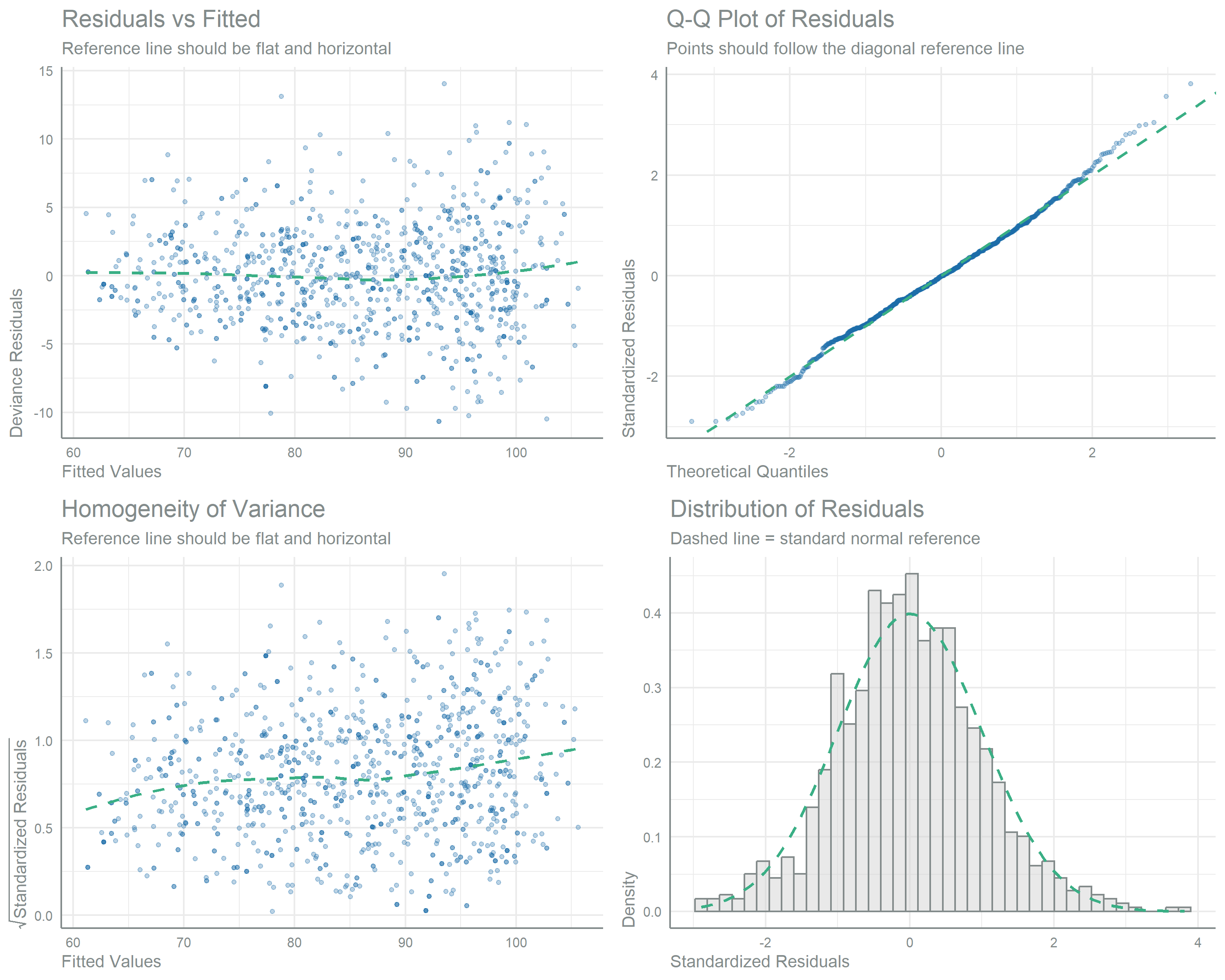
The four panels read as follows: residuals against fitted values show no systematic curvature, the Q-Q plot follows the diagonal with minor departures at the tails, the scale-location plot is approximately flat, and the residual histogram tracks the standard normal reference.
Smooth Term Partial Effects
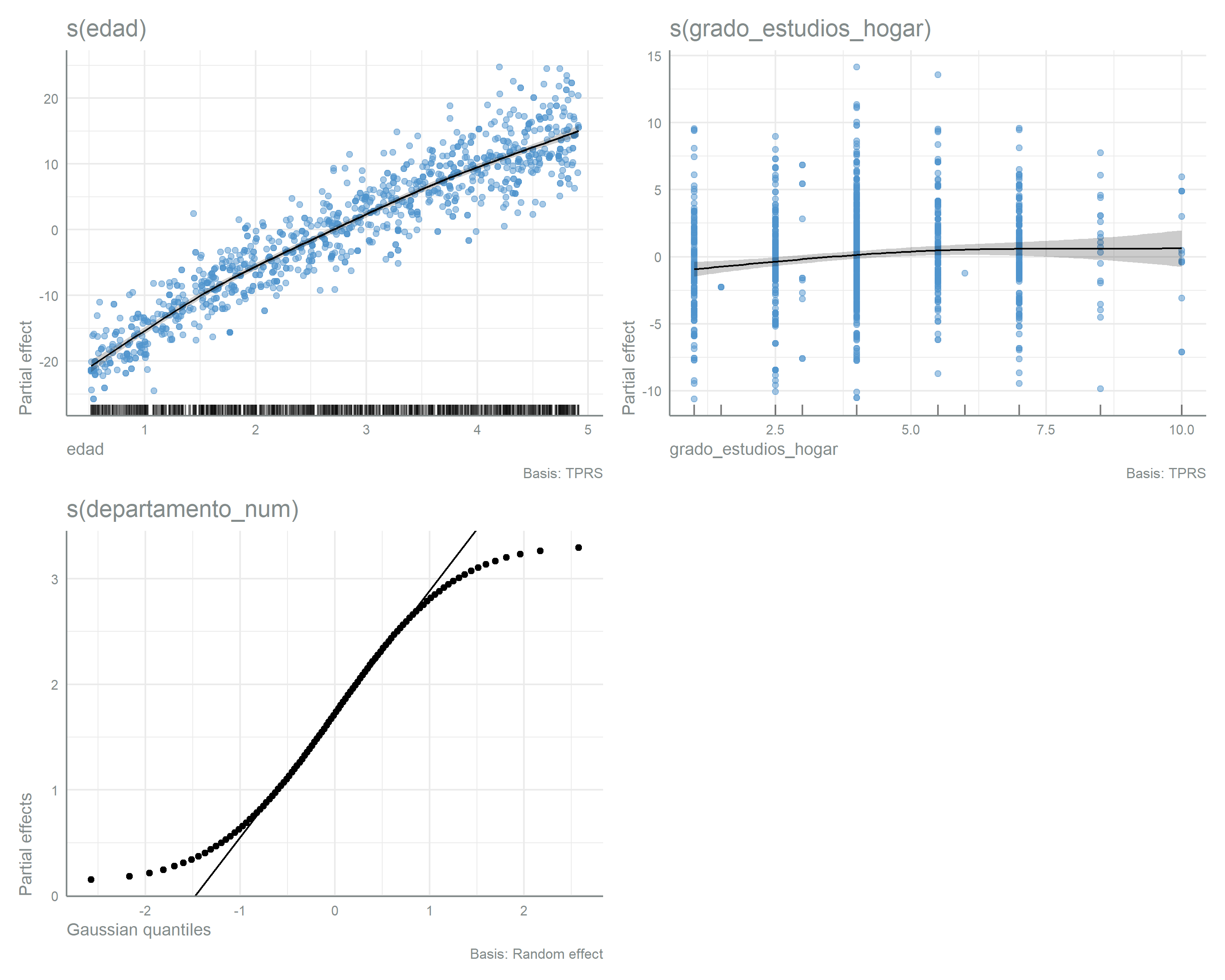
The age partial effect shows the decelerating growth curve: a steep positive slope from 6 to around 24 months that flattens through 59 months. The parental education smooth shows a weak positive gradient. The department panel is a Q-Q plot of the random-effect term against the normal distribution.
Concurvity Assessment
| Pairwise Concurvity (values > 0.3) | ||
| GAM analogue of multicollinearity between smooth terms | ||
| Term | Against | Concurvity1 |
|---|---|---|
| para | s(departamento_num) | 0.722 |
| s(departamento_num) | para | 0.722 |
| 1 Values > 0.8 (red) indicate high concurvity requiring attention. | ||
NoteConcurvity
The highest pairwise concurvity is 0.722, between the department term and the parametric block, below the 0.8 value at which the table flags a term. Geographic location and socioeconomic indicators are correlated in Guatemala, so some overlap between the two is expected. No term is removed on concurvity grounds.
Observed vs Fitted (Full Model)
Summary
Key Findings
Model fit: The GAM accounts for 89.3% of deviance (Adj. R² = 0.889) with three significant smooth terms and parametric predictors covering demographic, geographic and household-asset dimensions.
Out-of-sample accuracy: Cross-validation gives RMSE = 3.85 cm and R² = 0.883, with a mean bias of -0.01 cm and fold-level RMSE between 3.55 and 4.82 cm.
Age dominance: The age smooth carries the non-linear growth curve, while sex and the socioeconomic predictors add discriminating information on top of it.
Shrinkage toward the conditional mean: Height is overpredicted by 2.72 cm on average for stunted children and underpredicted by 2.18 cm for the rest. The quantile mapping applied downstream restores the spread of the distribution.
WarningLimitations
Training sample size — 773 original observations, 1,041 after expansion by survey weights, is a modest base for a GAM with 15 predictors and three smooth terms.
Age-dependent accuracy — RMSE rises from 3.25 cm in the 6-11 month group to 4.69 cm in the 48-59 month group, following the greater spread of height at older ages.
Departmental coverage — 5 departments carry an RMSE more than one standard deviation above the departmental mean, in two cases with a mean bias above 1.7 cm.
Cross-survey transfer assumption — The model assumes that the height-socioeconomic relationship in SIVESNU 2018, a health centre sample, holds in ENCOVI 2023, a household survey. The sampling frame difference is addressed by the calibration in transferring height to ENCOVI.
Application
The trained GAM is applied in transferring height to ENCOVI to predict height for ENCOVI 2023 children from their socioeconomic profiles. Those predictions are calibrated and converted into individual height-for-age z-scores through the WHO LMS reference tables, which is what the Meta-analysis (Gunaratna) pathway needs to estimate the change in stunting under biofortified maize adoption.