| Variable Audit Summary by Source Table | |||||
| Outcome distribution after audit against operational dictionary | |||||
| Table | Clean | Recoded | Passthrough | Not in dict. | Values recoded |
|---|---|---|---|---|---|
| hogar | 231 | 0 | 22 | 0 | 0 |
| miembros | 10 | 0 | 3 | 0 | 0 |
| mujer | 459 | 0 | 28 | 0 | 0 |
| nino | 430 | 3 | 14 | 0 | 9 |
| Audit rule: values outside the declared domain (factor levels for categorical, [min, max] for numeric) are replaced with NA. Variables flagged ‘Not in dict.’ should be reviewed for inclusion. | |||||
Preparing Stunting Modeling Data
Module 4: Covariate Prediction
Overview
Predicting child stunting requires combining anthropometric outcomes with demographic, socioeconomic, and health-related predictors. Survey datasets like SIVESNU contain hundreds of potential variables, but effective modeling requires a curated subset that balances predictive power with parsimony.
The challenge is threefold: (1) many variables have missing values that could bias results, (2) groups of related variables are highly correlated and redundant, and (3) not all variables contribute meaningful predictive information. This module implements a systematic, transparent selection pipeline that addresses each challenge while keeping every transformation traceable.
Before the merge, each SIVESNU source table is independently audited against an operational data dictionary that declares the universe of valid values for every variable. Out-of-domain values are recoded to NA so that all downstream stages operate on data whose semantic domain is fully under control.
By combining multiple SIVESNU 2018 tables — child anthropometrics, household characteristics, maternal factors, and the nutrient intake estimates from previous modules — we build a unified analytical dataset optimized for stunting prediction.
Target Population
Children aged 6-59 months with valid anthropometric measurements. Children under 6 months are excluded because exclusive breastfeeding is recommended during this period, making dietary intake patterns non-comparable to older children who consume complementary foods.
Data Integration Strategy
The base dataset — containing nutrient intake estimates, bioavailability adjustments, and FIES scores from previous pipeline steps — is merged with additional SIVESNU 2018 tables to create a comprehensive predictor set:
| Table | Contents | Purpose |
|---|---|---|
| Child | stunting, HAZ, vaccination, health controls, illness history | Outcomes and child-level predictors |
| Household | Assets, infrastructure, cooking fuel, altitude | Socioeconomic predictors |
| Women | Maternal education, age, physiological state | Maternal predictors |
| Members | Occupation classification | Agricultural exposure indicators |
Data Dictionary Audit
Each source table is audited independently against an operational data dictionary that declares, for every variable in the table, its type (factor, binary, numeric continuous, numeric integer, identifier, date, text) and its universe of valid values (factor levels for categorical variables, plausible numeric bounds for continuous and integer variables). Character columns are loaded with whitespace trimming applied uniformly, normalizing fixed-width string padding inherited from the original survey exports.
The audit applies a single rule: any value outside the declared universe is replaced with NA. Empty strings in character columns are normalized to NA before the comparison. The rule is applied uniformly regardless of whether out-of-domain values correspond to documented non-response codes, sentinel values, or artefacts from upstream transformations. Each table is audited against its own dictionary subset, so variables that share names across tables but use different encodings are validated against the universe corresponding to their actual source.
Audit Summary by Source Table
The audit returns four outcomes per variable:
- Clean: no out-of-domain values, no recoding required.
- Recoded: variable in the dictionary, at least one value fell outside the declared domain and was replaced with NA.
- Passthrough: identifier, date, or text variable explicitly exempted from domain validation.
- Not in dictionary: variable present in the data but absent from the dictionary, passed through unchanged and flagged for review.
Variables With Recoding Incidents
This table lists variables where the audit recoded at least one value, sorted by number of values replaced. Variables not in the dictionary appear in a separate block at the end and are highlighted for review.
| Per-Variable Audit Incidents | ||||||||
| Variables with out-of-domain recodings and variables absent from the dictionary | ||||||||
| Table | Variable | Type | N Total | NA (pre) | Recoded | NA (post) | % Recoded | Status |
|---|---|---|---|---|---|---|---|---|
| nino | edad_mes | numeric_integer | 902 | 3 | 2 | 5 | 0.22% | recoded |
| nino | intervalo | numeric_continuous | 902 | 491 | 1 | 492 | 0.11% | recoded |
| nino | pesoropanino | numeric_continuous | 902 | 883 | 1 | 884 | 0.11% | recoded |
| Recoded: variable in the dictionary, the indicated count of values fell outside the declared domain and was replaced with NA. Not in dictionary: variable present in the data but absent from the operational dictionary, passed through unchanged. |
||||||||
Merge Validation
Validate the merge process by examining record counts and match rates at each integration stage. The base dataset already contains the target population (children 6-59 months), so no additional age filtering is required.
| Phase A: Data Integration Summary | |||
| Record counts at each merge stage (audited tables) | |||
| Integration Stage | N Records | Change | % of Base |
|---|---|---|---|
| Base dataset (from 04_04) | 815 | — | 100.0% |
| Unique children in base | 789 | −26 | 96.8% |
| After household-level merges (hogar, mujer, ocupacion) | 815 | 26 | 100.0% |
| After child-level merge with deduplication | 789 | −26 | 96.8% |
| With valid outcomes (HFA & ZLEN) | 751 | −38 | 92.1% |
| Note: Base dataset duplicates (same nboletahogar/conglomerado/edad_an/sexo) are resolved during child-level merge. Source tables are audited individually before this merge. | |||
Variable Selection Pipeline
Survey datasets often contain hundreds of variables, many of which are redundant, have excessive missing values, or provide minimal predictive value. The selection pipeline narrows that pool to a parsimonious, informative predictor set.
The pipeline follows seven sequential steps:
| Step | Method | Purpose |
|---|---|---|
| 1 | Missing filter (>35%) | Exclude unreliable variables |
| 2 | Near-zero variance | Remove constant/near-constant variables |
| 3 | Random Forest imputation | Handle remaining missing values |
| 4 | Block PCA | Reduce dimensionality of correlated groups |
| 5 | Correlation filter (r>0.85) | Remove redundant predictors |
| 6 | Boruta selection | Identify relevant predictors |
| 7 | VIF verification | Confirm no multicollinearity (VIF < 5) |
NoteProtected Variables
Two variable sets are protected throughout the selection process: assignment variables (required for biofortified maize targeting: department, urban/rural, occupation, FIES score) and nutritional variables (the intake estimates that will be modified in biofortification scenarios). These participate in selection for assessment but are always retained regardless of results.
Candidate Variables Summary
| Phase B: Candidate Variable Summary | |
| Variable counts before and after exclusions | |
| Category | Count |
|---|---|
| Final | |
| Total columns in modeling dataset | 1,261 |
| Candidate variables for selection | 1,140 |
| Exclusions | |
| Header variables (excluded) | 7 |
| Outcome variables (excluded) | 2 |
| Design exclusions (excluded) | 79 |
Missing Values Analysis
Variables with excessive missing values (>35%) are excluded before imputation. This threshold balances information retention with imputation reliability — variables with higher missingness cannot be reliably imputed without introducing substantial uncertainty.
| Missing Values Analysis | |
| Distribution of candidate variables by missing rate | |
| Category | Count |
|---|---|
| Total variables | 1140 |
| Complete (0% missing) | 264 |
| Low missing (0-10%) | 268 |
| Moderate missing (10-35%) | 148 |
| High missing (>35%) | 460 |
| Threshold: Variables with >35% missing will be excluded from selection pipeline | |
Near-Zero Variance Filter
Variables with minimal variation provide little discriminatory power for prediction. The near-zero variance filter identifies variables where one value dominates (frequency ratio > 19) or there are very few unique values relative to sample size (< 10%).
| Near-Zero Variance Analysis | |
| Distribution of variables by variance characteristics | |
| Category | Count |
|---|---|
| Total variables analyzed | 680 |
| Zero variance | 43 |
| Near-zero variance | 173 |
| Adequate variance | 464 |
| Criteria: freqRatio > 19 and percentUnique < 10% | |
| Phase C: Variable Quality Filtering | |
| Sequential application of missing value and variance filters | |
| Stage | Count |
|---|---|
| Missing Values Filter | |
| Initial candidate variables | 1,140 |
| Excluded by missing filter (>35%) | 460 |
| Remaining after missing filter | 680 |
| Near-Zero Variance Filter | |
| Excluded by NZV filter | 216 |
| Final candidate variables for modeling | 464 |
| Thresholds: Missing >35% excluded; NZV per caret::nearZeroVar defaults | |
Missing Value Imputation
Variables that passed the quality filters may still have missing values (up to 35%). Random Forest-based multivariate imputation handles these gaps by predicting missing values from observed patterns across all variables, preserving complex relationships in the data.
Implementation uses the impute_rf_parallel() utility function, which wraps missRanger with a multi-threaded ranger engine and returns imputed values alongside out-of-bag error estimates (OOBE for continuous variables, PFC for categorical).
| Pre-Imputation Missing Values Assessment | |
| Candidate variables after Phase C filtering | |
| Metric | Value |
|---|---|
| Total candidate variables | 464 |
| Variables with no missing | 143 |
| Variables with missing values | 321 |
| Total cells in matrix | 348,464 |
| Total missing cells | 25,962 |
| Overall missing rate | 7.5% |
| Method: Random Forest-based multivariate imputation | |
| Random Forest Imputation Results | ||
| Out-of-bag error estimates | ||
| Metric | Value | Assessment |
|---|---|---|
| Variables imputed | 464 | — |
| Observations | 751 | — |
| OOBE | 0.4667 | Acceptable |
| PFC | 0.1921 | Acceptable |
| OOBE: aggregated out-of-bag error, continuous variables; acceptable below 0.50 PFC: Proportion Falsely Classified, categorical variables; acceptable below 0.20 |
||
Completion of Residual Missing Values
The Random Forest imputation engine can leave a residual NaN for a small subset of rows when the out-of-bag prediction collapses inside a terminal node with zero within-leaf variance. This affects continuous discrete-scale predictors.
Downstream analyses (block PCA, correlation filter, Boruta, VIF) operate on a complete predictor matrix, so residual missing values are completed with a variable-specific rule:
- Numeric / integer variables: median of the observed values. The median preserves the support of discrete-scale ordinal variables, which the mean does not.
- Factor variables: mode of the observed values.
Completing rather than discarding keeps every record in the modeling dataset. The count of values completed by each rule is reported in the table below.
| Residual Missing Value Completion | ||
| Values completed by variable-specific rule after RF imputation | ||
| Variable | N Completed | Completion Rule |
|---|---|---|
| — Residual NAs after completion — | 0 | Integrity check: passed |
TipImputation Quality
The out-of-bag error estimates indicate acceptable imputation quality. Out-of-bag (OOB) error estimates are calculated from observations that were randomly excluded during tree construction within the Random Forest algorithm, providing an internal quality metric for imputed values without requiring a separate test set. Random Forest imputation preserves variable relationships better than simpler methods like mean/mode imputation, which is essential for accurate downstream modeling.
| Phase D: Imputation Summary | |
| Random Forest-based missing value imputation | |
| Stage | Value |
|---|---|
| Candidate variables entering imputation | 464 |
| Observations | 751 |
| Missing cells before imputation | 25,962 |
| Missing cells after imputation | 0 |
Imputation method: impute_rf_parallel() (missRanger + ranger engine) |
|
Block PCA: Dimensionality Reduction
Many SIVESNU variables capture related constructs — vaccination records, wealth indicators, health monitoring visits, and morbidity symptoms. These variable groups exhibit high internal correlation, which can destabilize regression models and obscure individual variable importance.
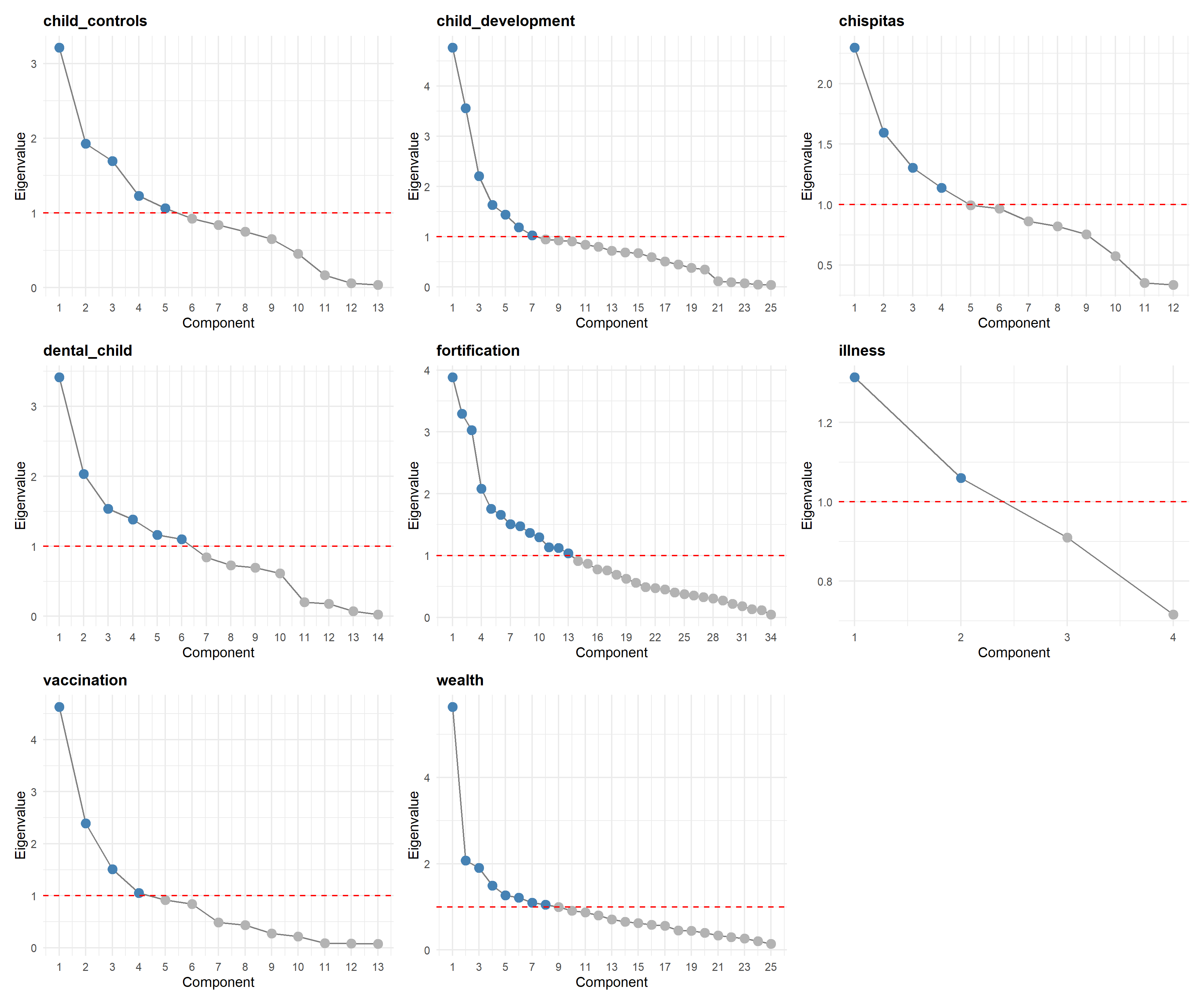
Block principal components analysis (PCA) transforms each conceptual group into orthogonal principal components, reducing dimensionality while preserving the majority of within-block variance. This approach yields interpretable composite scores (e.g., “vaccination coverage”, “household wealth”) rather than dozens of intercorrelated individual variables.
| PCA Block Definitions | |||
| Variable groups for dimensionality reduction | |||
| Block | Description | N Variables | Sample Variables |
|---|---|---|---|
| vaccination | Child vaccination profile | 13 | hepb_1, neumo_1, rota_2 |
| wealth | Household wealth indicators | 25 | material_paredes, material_techo, material_piso |
| child_controls | Child health check-ups | 13 | control_temp_oido, control_carnet_antro, control_numero_peso_noreg |
| fortification | Fortified food consumption | 34 | fortif_pdulce, fortif_pdulce_dias, fortif_pdulce_veces |
| chispitas | Chispitas supplementation behavior | 12 | chispitas_vez, chispitas_no6mes_noservicios, chispitas_donde |
| illness | Recent illness indicators | 4 | diarrea_sabe_vacuna, diarrea_tenido_2semanas, tos_tenido_2semanas |
| child_development | Child development milestones | 25 | di_libros, di_juega_juguetes_cas, di_juega_juguetes_fab |
| dental_child | Child dental health | 14 | dientes_limpia_vezdia, dientes_consulta_lab, dientes_consulta_clin |
| Note: Blocks with <3 variables (highlighted) will not undergo PCA | |||
| Block PCA Dimensionality Reduction | |||||
| Variance preserved while reducing variable count | |||||
| Block | Description | Original Variables | Components Retained | Variance Retained (%) | Reduction (%) |
|---|---|---|---|---|---|
| vaccination | Child vaccination profile | 13 | 4 | 73.7 | 69 |
| wealth | Household wealth indicators | 25 | 8 | 63.0 | 68 |
| child_controls | Child health check-ups | 13 | 5 | 70.2 | 62 |
| fortification | Fortified food consumption | 34 | 13 | 72.5 | 62 |
| chispitas | Chispitas supplementation behavior | 12 | 4 | 52.8 | 67 |
| illness | Recent illness indicators | 4 | 2 | 59.4 | 50 |
| child_development | Child development milestones | 25 | 7 | 63.3 | 72 |
| dental_child | Child dental health | 14 | 6 | 76.0 | 57 |
| TOTAL | 140 | 49 | — | 65 | |
| Method: Principal Component Analysis with Kaiser criterion (eigenvalue > 1) Color coding: Green ≥70%, Orange 60-70%, Red <60% variance retained |
|||||
| Phase E: Candidate Variable Transformation | |
| Block PCA dimensionality reduction on candidate variables | |
| Metric | Value |
|---|---|
| Candidate variables post-NZV | 464 |
| — Variables in PCA blocks (transformed) | 140 |
| — Variables not in blocks (kept as-is) | 324 |
| PCA components created | 49 |
| Candidate variables after PCA | 373 |
| Assignment variables preserved | 7 of 7 |
| Criterion: Kaiser rule (eigenvalue > 1) with minimum 1 component per block | |
TipDimensionality Reduction
Block PCA achieved substantial dimensionality reduction while preserving the majority of variance within each conceptual domain. The vaccination and wealth blocks show particularly high variance retention, indicating that these constructs are well-captured by their principal components.
Feature Selection
With dimensionality reduced, we now identify which variables — both individual predictors and PCA components — contribute meaningfully to stunting prediction. This three-step process removes redundancy and identifies the most informative predictors.
Correlation Filter
Highly correlated variables (r > 0.85) provide redundant information and can inflate coefficient standard errors. The correlation filter removes the variable with higher mean absolute correlation from each highly correlated pair.
| Correlation Filter Results | |
| Removal of redundant variables (high pairwise correlation) | |
| Metric | Value |
|---|---|
| Variables entering correlation filter | 373 |
| Correlation threshold | r > 0.85 |
| Highly correlated variables identified | 51 |
| Protected assignment variables (kept) | 3 |
| Variables removed | 48 |
| Variables retained | 325 |
| Method: caret::findCorrelation removes variable with higher mean absolute correlation from each pair | |
Boruta Feature Selection
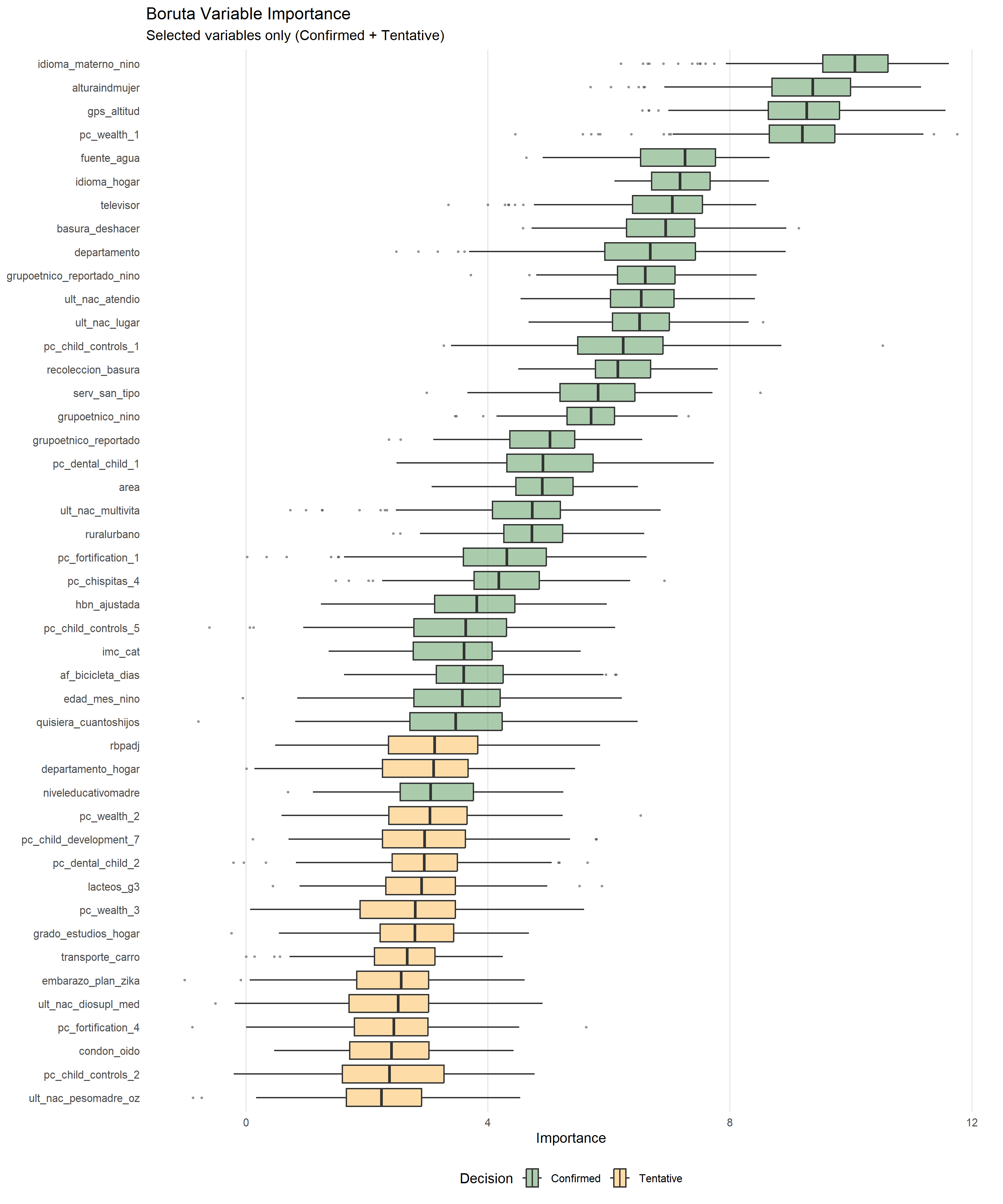
Boruta identifies variables with confirmed predictive importance by comparing each variable’s Random Forest importance against “shadow” variables (permuted copies of the original predictors). Variables consistently outperforming their shadows are classified as Confirmed; those consistently worse are Rejected.
The implementation runs with a multi-threaded ranger engine (via Boruta::getImpRfZ) for efficient computation. Feature selection uses HAZ (continuous z-score) rather than binary stunting status to preserve full distributional information — since stunting is simply HAZ dichotomized at -2, selecting on HAZ captures identical predictive relationships without information loss.
| Boruta Feature Selection Results | |
| Variable importance assessment for HAZ prediction | |
| Metric | Value |
|---|---|
| Variables evaluated | 325 |
| Confirmed (relevant) | 30 |
| Tentative (borderline) | 15 |
| Rejected (not relevant) | 280 |
| Variables selected (Confirmed + Tentative) | 45 |
| Method: Boruta with ranger Random Forest engine (Z-score importance) | |
ImportantVariables Selected
Boruta identified the most relevant predictors for the continuous HAZ outcome, including child age, maternal characteristics, food security indicators, and several PCA components capturing vaccination coverage, household wealth, and child health monitoring patterns.
VIF Verification
Variance Inflation Factor (VIF) assesses multicollinearity across the selected predictors. The correlation filter addressed pairwise correlations; VIF detects multicollinearity arising from linear combinations of several variables. For categorical variables the generalized VIF is adjusted by degrees of freedom, so every variable is reported on a comparable scale.
Variables above the high threshold of 10 are pruned iteratively: at each step the one with the lowest Boruta median importance among them is dropped and the VIF is recomputed on the remaining set. A construct captured through two separate survey items passes the pairwise correlation filter while still inflating the variance of both coefficients, and this step resolves those cases, keeping whichever member carries more signal on the outcome.
| Phase F3: VIF Verification Summary | |
| Multicollinearity check on Boruta-selected variables | |
| Metric | Value |
|---|---|
| Variables evaluated | 43.00 |
| Acceptable (VIF ≤ 5) | 43.00 |
| Moderate (5 < VIF ≤ 10) | 0.00 |
| High (VIF > 10) | 0.00 |
| Maximum VIF | 4.91 |
| Mean VIF | 2.03 |
| Method: VIF with GVIF adjustment for categorical variables | |
| Variance Inflation Factor Analysis | ||
| Multicollinearity assessment for selected predictors | ||
| Variable | VIF | Status |
|---|---|---|
| grupoetnico_reportado_nino | 4.91 | Acceptable |
| idioma_hogar | 4.60 | Acceptable |
| basura_deshacer | 4.49 | Acceptable |
| pc_wealth_1 | 3.93 | Acceptable |
| grupoetnico_reportado | 3.89 | Acceptable |
| idioma_materno_nino | 3.50 | Acceptable |
| grupoetnico_nino | 3.41 | Acceptable |
| recoleccion_basura | 3.34 | Acceptable |
| ult_nac_atendio | 2.75 | Acceptable |
| area | 2.59 | Acceptable |
| serv_san_tipo | 2.58 | Acceptable |
| ult_nac_lugar | 2.57 | Acceptable |
| televisor | 2.31 | Acceptable |
| edad_mes_nino | 2.16 | Acceptable |
| fuente_agua | 1.95 | Acceptable |
| alturaindmujer | 1.81 | Acceptable |
| grado_estudios_hogar | 1.75 | Acceptable |
| pc_wealth_2 | 1.72 | Acceptable |
| pc_dental_child_1 | 1.70 | Acceptable |
| niveleducativomadre | 1.66 | Acceptable |
| pc_wealth_3 | 1.65 | Acceptable |
| departamento | 1.61 | Acceptable |
| hbn_ajustada | 1.58 | Acceptable |
| condon_oido | 1.43 | Acceptable |
| pc_child_controls_1 | 1.42 | Acceptable |
| ult_nac_diosupl_med | 1.39 | Acceptable |
| pc_child_controls_5 | 1.38 | Acceptable |
| lacteos_g3 | 1.35 | Acceptable |
| transporte_carro | 1.35 | Acceptable |
| pc_fortification_1 | 1.27 | Acceptable |
| af_bicicleta_dias | 1.24 | Acceptable |
| quisiera_cuantoshijos | 1.21 | Acceptable |
| ult_nac_pesomadre_oz | 1.21 | Acceptable |
| pc_dental_child_2 | 1.19 | Acceptable |
| departamento_hogar | 1.19 | Acceptable |
| rbpadj | 1.18 | Acceptable |
| ult_nac_multivita | 1.17 | Acceptable |
| embarazo_plan_zika | 1.16 | Acceptable |
| pc_child_controls_2 | 1.16 | Acceptable |
| pc_fortification_4 | 1.15 | Acceptable |
| pc_child_development_7 | 1.12 | Acceptable |
| imc_cat | 1.11 | Acceptable |
| pc_chispitas_4 | 1.08 | Acceptable |
| Thresholds: VIF > 10 high multicollinearity; VIF > 5 moderate concern | ||
| Variables Removed by VIF Pruning | ||
| Lowest Boruta median importance among those above the threshold | ||
| Variable | VIF at removal | Boruta median importance |
|---|---|---|
| ruralurbano | 171.53 | 4.73 |
| gps_altitud | 28.70 | 9.27 |
| Removed in the order shown; the VIF is the value held at the iteration of removal | ||
TipMulticollinearity Assessment
The pruning removed 2 variables: ruralurbano, gps_altitud. Each was the less important member of a pair measuring the same construct — the urban/rural classification, recorded in two separate survey items, and two altitude measurements.
The 43 variables that remain all sit at or below the acceptable threshold of 5, with a maximum of 4.91.
Final Output
The pipeline produces two key datasets and transformation objects required for downstream modeling and scenario simulation.
| Phase G: Output Files Summary | ||||
| Files generated for downstream analysis | ||||
| File | Location | Description | Contents | Purpose |
|---|---|---|---|---|
| 04_05_sivesnu_stunting_modeling.parquet | transfer/ | Training dataset with selected predictors + PCA components | 751 obs × 96 vars | Model training (Phase 4) |
| 04_05_sivesnu_pre_pca.parquet | transfer/ | Pre-PCA dataset for synthetic population generation | 751 obs × 1261 vars | Synthetic population generation |
| 04_05_pca_transforms.rds | models/ | PCA transformation objects (prcomp) for each block | 8 PCA block transforms | Apply PCA to synthetic data via predict() |
| 04_05_pca_block_definitions.rds | models/ | Block definitions (variable lists per block) | 8 block definitions | Identify variables per block |
| 04_05_boruta_selected_variables.rds | models/ | Boruta-selected variables (Confirmed + Tentative) | 45 variables | Automated formula construction in 04_06 / 04_07 |
| 04_05_selected_variables.rds | models/ | Variable selection results at each pipeline stage | 10 variable vectors | Documentation and downstream reference |
| All files saved relative to project root via here() | ||||
| Variable Selection Pipeline Summary | |||
| Complete processing workflow from raw data to final predictors | |||
| Phase | Input | Output | Method |
|---|---|---|---|
| A1-A2. Data Loading | Base dataset + SIVESNU tables | 815 base observations | read_parquet + clean_names + zap_* |
| A3. Dictionary Audit | Loaded SIVESNU tables | Out-of-domain values recoded to NA | Domain-only validation per source table |
| A4. Data Merge | Audited SIVESNU tables + base dataset | 789 observations | Fuzzy merge on household + age ± 1 + sex |
| B. Variable Classification | Merged dataset | 7 header + 2 outcome | Pattern-based classification |
| C1. Missing Values Filter | All candidate variables | 680 variables retained | > 35% NA threshold |
| C2. Near-Zero Variance Filter | Post-missing variables | 464 variables retained | caret::nearZeroVar |
| D. Imputation (Random Forest) | Post-NZV variables | Complete data (no NAs) | Random Forest (impute_rf_parallel, ntree=50, maxiter=5) |
| E. Block PCA | Imputed variables | 49 PCA components | Kaiser criterion (eigenvalue > 1) |
| F1. Correlation Filter | Post-PCA variables | 325 variables retained | caret::findCorrelation (r > 0.85) |
| F2. Boruta Selection | Post-correlation variables | 45 variables selected | Boruta on ZLEN (maxRuns=150, ranger engine) |
| F3. VIF Verification | Post-Boruta variables | 43 variables verified | car::vif (GVIF adjustment) |
| G. Final Output | Final predictor set | 88 final predictors | Union: Boruta + assignment + nutritional |
Summary
Pipeline Overview
This module transformed raw SIVESNU 2018 data into a modeling-ready dataset through a systematic, reproducible pipeline. Starting from multiple survey tables, we audited each source independently, integrated child, household, maternal, and occupation data, then applied rigorous variable selection to identify the most relevant predictors for stunting.
Key Results
| Stage | Output |
|---|---|
| Data integration | 751 children with valid outcomes |
| Dictionary audit | 3 variables with out-of-domain recodings; 9 values recoded to NA |
| Imputation OOB error | OOBE = 0.4667; PFC = 0.1921 |
| Boruta selection | 45 variables retained for HAZ prediction |
| VIF verification | 43 of 43 variables with acceptable multicollinearity |
Methodological Notes
Dictionary audit — Each SIVESNU source table is validated independently against an operational data dictionary before the merge. Out-of-domain values are recoded to NA so downstream stages operate on data whose semantic domain is fully under control.
Missing value threshold (35%) — Variables exceeding this threshold cannot be reliably imputed without introducing substantial uncertainty. The threshold follows Van Buuren (2018) and Madley-Dowd et al. (2019) and balances information retention with imputation reliability.
Boruta on HAZ — Feature selection used the continuous outcome rather than the binary classification to preserve full distributional information. Since stunting is HAZ dichotomized at -2 SD, selecting on HAZ captures identical predictive relationships.
Block PCA — Conceptually related variables (vaccination, wealth, health monitoring) were reduced to principal components. This approach preserves construct-level interpretability while eliminating within-block multicollinearity.
Protected variables — Assignment variables (department, urban/rural, occupation, FIES) and nutritional estimates are always retained regardless of selection results, as they are required for biofortification targeting and scenario simulation.
Application
The outputs from this module enable:
- Stunting model development — Training the continuous HAZ regression model, with the binary stunting classification derived directly from the predicted HAZ values.
- Synthetic population generation — Creating representative populations for scenario modeling using the pre-PCA dataset.
- Biofortification simulation — Modifying nutritional variables while preserving covariate structure.