Continuous Stunting Model

Module 4: Covariate Prediction

Overview

The continuous Z-score model predicts the magnitude of height-for-age deviation (HAZ) from the WHO reference. Modeling HAZ directly rather than the binary stunting classification (stunted = HAZ < -2) preserves the full distributional information about child growth, since the WHO threshold is a direct transformation of the same z-score. The continuous outcome serves two purposes:

Distributional analysis — Understand how far children fall below growth standards, not just whether they cross the −2 SD threshold.
Impact quantification — Estimate the expected Z-score improvement from biofortification, enabling comparison with other nutritional interventions.

This approach is particularly valuable for biofortification impact assessment because improvements in nutrient intake may shift children’s Z-scores without necessarily crossing the stunting threshold. Capturing these sub-threshold improvements provides a more complete picture of intervention effects.

The binary stunting classification is derived afterwards by thresholding both the observed and the predicted z-scores at −2, which lets us evaluate the continuous model as a binary classifier of stunting status without fitting a separate logistic regression.

Data Preparation

Training Data and Normalization Parameters

The model uses the prepared SIVESNU dataset from the previous module. The nutritional index components are normalized using z-score parameters (mean and SD) calculated on the outlier-treated training data; these parameters are exported and reused downstream in scenario simulation, so that biofortified values are projected onto the exact same scale as the training data.

Outlier Treatment

Outlier treatment is directional and stratified by household food insecurity. Children are grouped into terciles of the FIES Rasch score, the measure of food access collected directly in SIVESNU and documented in FIES Food Security Score. Within the most food-insecure tercile, upper outliers are pulled down to the stratum median; within the most food-secure tercile, lower outliers are pulled up to the stratum median. The intermediate tercile is left untouched.

An intake estimate that is extreme relative to a household’s observed food access carries the uncertainty of the transfer model prediction that produced it. Bounding those values limits their influence on the z-score normalization parameters, which set the scale of the composite index.

Stratifying Variable

The stratification uses food access, which is observed independently of the anthropometric outcome. The outcome itself takes no part in the treatment, so the corrected values carry no imprint of the height-for-age z-scores the model goes on to predict.

Nutritional Index Construction

The composite nutritional index combines six bioavailable nutrient measurements into a single predictor using z-score normalization with equal weights:

Component	Units	Role
Iron (absorbed)	mg/day	Micronutrient — biofortification target
Zinc (TAZ, Miller equation)	mg/day	Micronutrient — biofortification target
Protein (PDCAAS-adjusted)	g/day	Macronutrient quality — biofortification target
Lysine	mg/day	Amino acid quality
Tryptophan	mg/day	Amino acid quality
Energy	kcal/day	Overall caloric adequacy

Why a Composite Index?

Individual nutrients are highly correlated — children with adequate iron intake typically have adequate zinc, protein, and energy intake. Including all six nutrients as separate predictors would cause multicollinearity, attenuating coefficient estimates and reducing sensitivity to biofortification effects. The composite index captures overall nutrient adequacy while maintaining a single coefficient that responds predictably to nutrient improvements.

Table 1: Z-score normalization parameters for nutritional index components

Nutritional Index: Z-Score Normalization Parameters. Calculated from outlier-treated SIVESNU training data
Nutrient Component	Mean (μ)	Std. Dev. (σ)
Nutritional Index: Z-Score Normalization Parameters
Calculated from outlier-treated SIVESNU training data
fe_absorbed_mg	0.5553	0.4522
taz_mg	1.1175	0.4264
prot_g_total	17.1679	16.8283
lys_mg_total	1.2844	1.1919
trp_mg_total	0.2620	0.2570
ene_kcal_total	1,121.7296	1,162.1837
Parameters saved to: 04_06_ni_zscore_normalization_params.rds

Multicollinearity Assessment

Before model fitting, we assess the correlation between the nutritional index and every Boruta-selected predictor present in the dataset. Variables highly correlated with the index (|r| > 0.45) could attenuate its coefficient through multicollinearity, reducing the model’s sensitivity to nutritional changes in simulation scenarios. The table below shows the ten predictors most correlated with the nutritional index; those exceeding the threshold are dropped from the model formula in the next phase. Mandatory predictors, including nutritional_index itself, bypass this filter.

Table 2: Correlation of Boruta-selected predictors with nutritional_index

Multicollinearity with Nutritional Index. Top 10 correlated predictors (exclusion threshold: |r| > 0.45)
Variable	Correlation (r)	Exclude
Multicollinearity with Nutritional Index
Top 10 correlated predictors (exclusion threshold: \|r\| > 0.45)
grado_estudios_hogar	0.531	Yes
pc_wealth_1	−0.379	No
pc_wealth_2	−0.369	No
televisor	−0.336	No
ult_nac_diosupl_med	0.327	No
pc_dental_child_1	−0.325	No
serv_san_tipo	−0.310	No
basura_deshacer	0.308	No
recoleccion_basura	−0.296	No
grupoetnico_reportado_nino	0.296	No
Variables flagged 'Yes' are dropped from the model formula in Phase B.

Model Specification

Predictor Structure

The model formula is constructed data-driven from the current state of the pipeline. No predictor list is hard-coded in this script; every term is the result of upstream selection and a univariate GAM evaluation:

Starting set: the Boruta-selected variables exported by the previous module.
Correlation filter: variables flagged as Exclude = Yes in the multicollinearity table are dropped to preserve the sensitivity of nutritional_index in simulation scenarios.
Mandatory inclusion: nutritional_index is always kept, bypassing the correlation filter.
Polynomial degree: for every numeric predictor, a univariate GAM is fitted against zlen and its effective degrees of freedom (edf) translate into the nearest admissible polynomial degree in {1, 2, 3}. Principal components (pc_*) are treated as linear by design, since polynomials on a linear combination of variables are not semantically meaningful.

Univariate GAM fits are parallelized through a local mirai pool for efficient execution.

Formula Construction Audit

The table below traces, variable by variable, the decision made by the formula builder. Two columns deserve special attention:

Action: the bucket the variable falls into.

dropped_correlation: Boruta-selected but dropped because its correlation with nutritional_index exceeds the exclusion threshold (|r| > 0.45). Flagged in pink.
forced_linear: variables forced to linear (polynomial degree 1) by the linear_only argument. Principal components are handled this way. Flagged in blue.
gam_inferred: numeric variables whose polynomial degree (1, 2 or 3) was determined from the effective degrees of freedom of a univariate GAM fitted against the outcome.
kept_categorical: factor variables, entered as categorical terms in the formula (no polynomial applicable).

GAM Status: the outcome of the univariate GAM evaluation.

ok: the GAM fitted cleanly and the polynomial degree was assigned from its edf.
forced: the variable bypassed the GAM (listed in linear_only); degree fixed at 1.
categorical: the variable is a factor; the GAM is not applicable.
fit_failed: the GAM call aborted (typically because a numeric predictor has too few distinct values for the spline basis). Degree falls back to 1. Variables that are conceptually categorical but stored as numeric codes (e.g. binary 1/2 codings) end up here; their treatment as linear is functionally equivalent to their categorical counterpart and does not affect the model.
edf_unavailable: the GAM fitted but returned a non-finite edf. Degree falls back to 1. Rare.

Table 3: Audit trail of formula construction decisions

Formula Construction Audit. Data-driven from Boruta + correlation filter + GAM edf
Variable	Source	Action	Polynomial Degree	GAM edf	GAM Status
Formula Construction Audit
Data-driven from Boruta + correlation filter + GAM edf
grado_estudios_hogar	boruta	dropped_correlation	—	—	excluded
pc_child_controls_1	boruta	forced_linear	1	—	forced
pc_child_controls_2	boruta	forced_linear	1	—	forced
pc_child_controls_5	boruta	forced_linear	1	—	forced
pc_child_development_7	boruta	forced_linear	1	—	forced
pc_chispitas_4	boruta	forced_linear	1	—	forced
pc_dental_child_1	boruta	forced_linear	1	—	forced
pc_dental_child_2	boruta	forced_linear	1	—	forced
pc_fortification_1	boruta	forced_linear	1	—	forced
pc_fortification_4	boruta	forced_linear	1	—	forced
pc_wealth_1	boruta	forced_linear	1	—	forced
pc_wealth_2	boruta	forced_linear	1	—	forced
pc_wealth_3	boruta	forced_linear	1	—	forced
alturaindmujer	boruta	gam_inferred	3	6.559	ok
edad_mes_nino	boruta	gam_inferred	3	3.435	ok
hbn_ajustada	boruta	gam_inferred	3	4.637	ok
idioma_hogar	boruta	gam_inferred	3	7.097	ok
nutritional_index	mandatory	gam_inferred	3	2.298	ok
quisiera_cuantoshijos	boruta	gam_inferred	3	3.329	ok
rbpadj	boruta	gam_inferred	3	2.402	ok
ult_nac_pesomadre_oz	boruta	gam_inferred	3	2.529	ok
af_bicicleta_dias	boruta	kept_categorical	—	—	categorical
area	boruta	kept_categorical	—	—	categorical
basura_deshacer	boruta	kept_categorical	—	—	categorical
condon_oido	boruta	kept_categorical	—	—	categorical
departamento	boruta	kept_categorical	—	—	categorical
departamento_hogar	boruta	kept_categorical	—	—	categorical
embarazo_plan_zika	boruta	kept_categorical	—	—	categorical
fuente_agua	boruta	kept_categorical	—	—	categorical
grupoetnico_nino	boruta	kept_categorical	—	—	categorical
grupoetnico_reportado	boruta	kept_categorical	—	—	categorical
grupoetnico_reportado_nino	boruta	kept_categorical	—	—	categorical
idioma_materno_nino	boruta	kept_categorical	—	—	categorical
imc_cat	boruta	kept_categorical	—	—	categorical
lacteos_g3	boruta	kept_categorical	—	—	categorical
niveleducativomadre	boruta	kept_categorical	—	—	categorical
recoleccion_basura	boruta	kept_categorical	—	—	categorical
serv_san_tipo	boruta	kept_categorical	—	—	categorical
televisor	boruta	kept_categorical	—	—	categorical
transporte_carro	boruta	kept_categorical	—	—	categorical
ult_nac_atendio	boruta	kept_categorical	—	—	categorical
ult_nac_diosupl_med	boruta	kept_categorical	—	—	categorical
ult_nac_lugar	boruta	kept_categorical	—	—	categorical
ult_nac_multivita	boruta	kept_categorical	—	—	categorical

Model Fitting

We use survey-weighted linear regression (Gaussian family) to predict continuous z-scores. The survey design accounts for SIVESNU’s cluster sampling with child-level weights (pesonino), so the coefficient estimates refer to the national population of children aged 6–59 months.

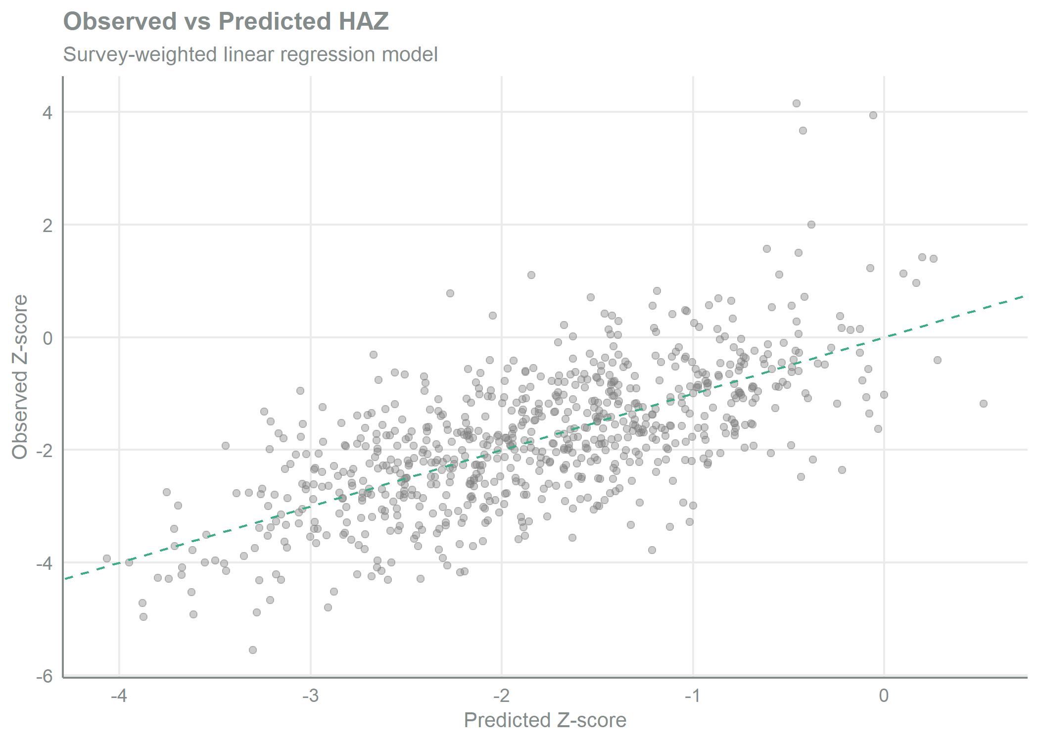
Model Discrimination

Good model performance appears as points clustering around the diagonal, indicating predicted values closely match observed Z-scores. Systematic deviations from the diagonal would suggest model misspecification or missing predictors.

Scatter plot with predicted height-for-age z-score on the x-axis and observed z-score on the y-axis, overlaid with a dashed diagonal reference line of perfect agreement. Points cluster in a broad cloud around the diagonal without systematic curvature or drift, indicating the survey- weighted linear model captures the overall relationship with no obvious misspecification, though scatter around the line reflects residual variability. — Figure 1: Observed vs predicted Z-scores

Model Evaluation

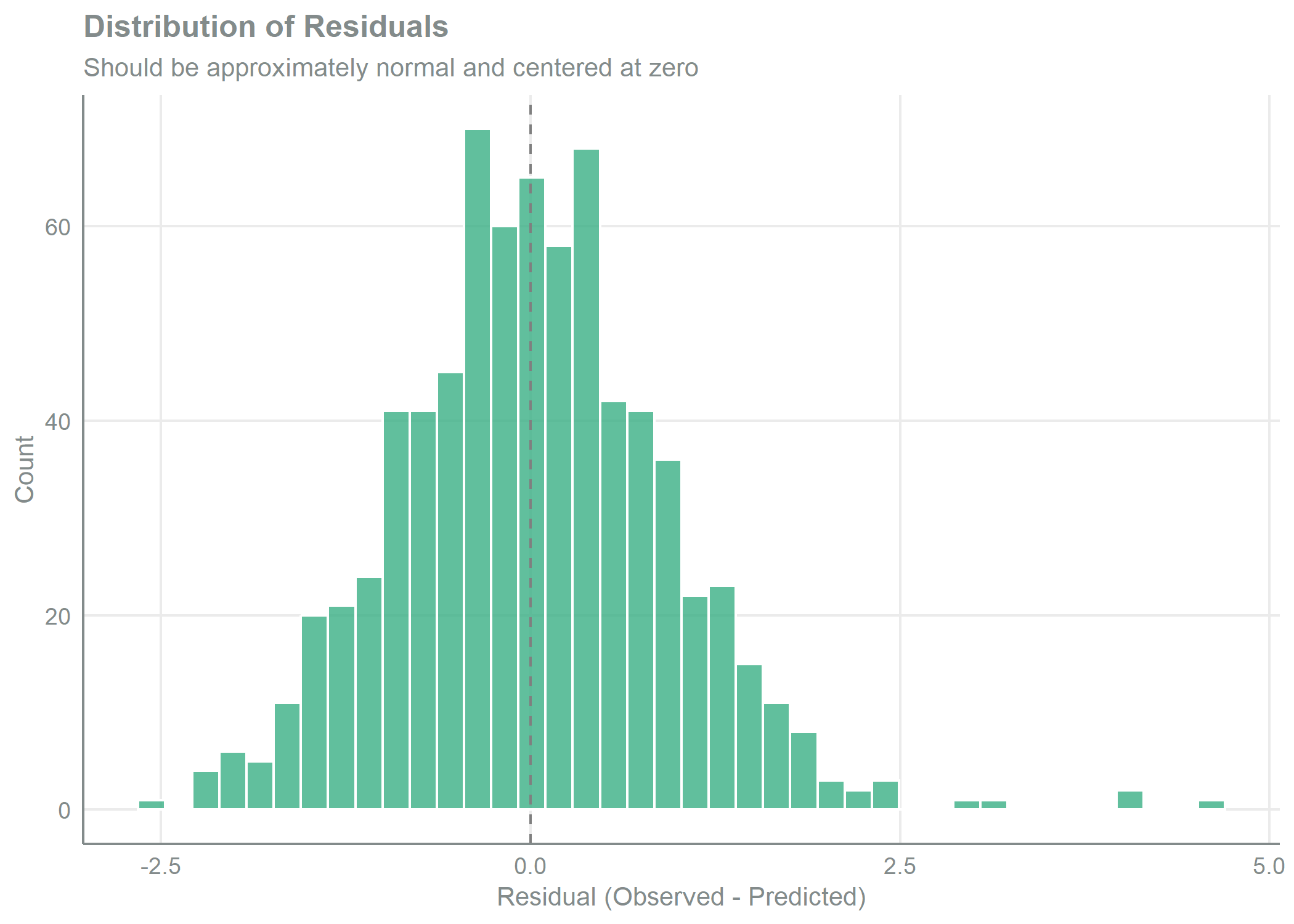
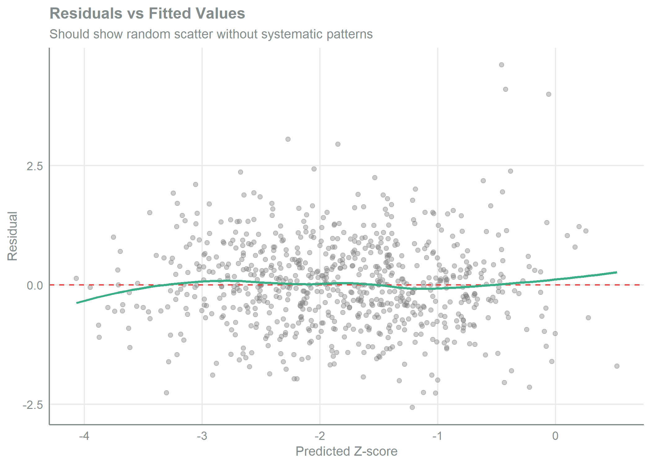
Residual Diagnostics

Linear regression assumes residuals are approximately normal and homoscedastic. The histogram should show a symmetric distribution centered at zero, while the residuals vs. fitted plot should display random scatter without systematic patterns. A flat loess smooth is what the linear specification predicts for the residual structure.

Histogram of model residuals (observed minus predicted z-score) on the x-axis and count on the y-axis, with a dashed vertical line at zero. The bars form a single symmetric bell-shaped mound centred on zero, consistent with the approximately normal, unbiased residuals that linear regression assumes. — Figure 2: Distribution of model residuals

Scatter plot with predicted z-score on the x-axis and residual on the y-axis, a dashed horizontal reference line at zero, and a loess smooth curve through the points. The points spread in a roughly even band around zero and the smooth stays close to flat, showing random scatter without systematic pattern and supporting the homoscedasticity and linearity assumptions. — Figure 3: Residuals vs fitted values

Performance Metrics

Table 4: Model performance metrics

HAZ Linear Regression Model Performance. Survey-weighted linear regression with polynomial terms
Metric	Value
HAZ Linear Regression Model Performance
Survey-weighted linear regression with polynomial terms
R²	0.445
RMSE	0.913
MAE	0.706
Observations	751

Binary Stunting Classification

The continuous HAZ model produces predictions on the height-for-age z-score scale. Stunting is defined by the WHO threshold HAZ < −2. By dichotomising both the observed and the predicted z-scores at this threshold, the continuous model is evaluated as a binary classifier of stunting status.

All metrics in this section are survey-weighted (pesonino) so that they reflect the population of children aged 6–59 months in Guatemala rather than the unweighted sample.

Derived Stunting Prevalence

Table 5: Observed vs predicted stunting prevalence

Stunting Prevalence: Observed vs Predicted. WHO threshold HAZ < −2
Metric	Value
Stunting Prevalence: Observed vs Predicted
WHO threshold HAZ < −2
Observations	751
Observed stunting prevalence (unweighted)	42.2%
Observed stunting prevalence (survey-weighted)	44.9%
Predicted stunting prevalence (survey-weighted)	45%

Survey-Weighted Confusion Matrix

Table 6: Survey-weighted confusion matrix at WHO threshold HAZ < −2

Survey-Weighted Confusion Matrix. Cell values are weighted counts (population estimates)
Observed \ Predicted	Not stunted	Stunted
Survey-Weighted Confusion Matrix
Cell values are weighted counts (population estimates)
Not stunted	326	88
Stunted	88	249

Classification Metrics

Table 7: Survey-weighted classification metrics at WHO threshold

Survey-Weighted Classification Metrics. Binary stunting classification at threshold HAZ < −2
Metric	Value	Interpretation
Survey-Weighted Classification Metrics
Binary stunting classification at threshold HAZ < −2
Accuracy	76.6%	Overall agreement between observed and predicted classification
Sensitivity (Recall)	74%	Proportion of stunted children correctly identified
Specificity	78.7%	Proportion of non-stunted children correctly identified
Positive Predictive Value (Precision)	73.8%	Probability that a child predicted as stunted is truly stunted
Negative Predictive Value	78.8%	Probability that a child predicted as non-stunted is truly non-stunted
F1 Score	0.739	Harmonic mean of precision and recall
Cohen's Kappa	0.527	Agreement beyond chance

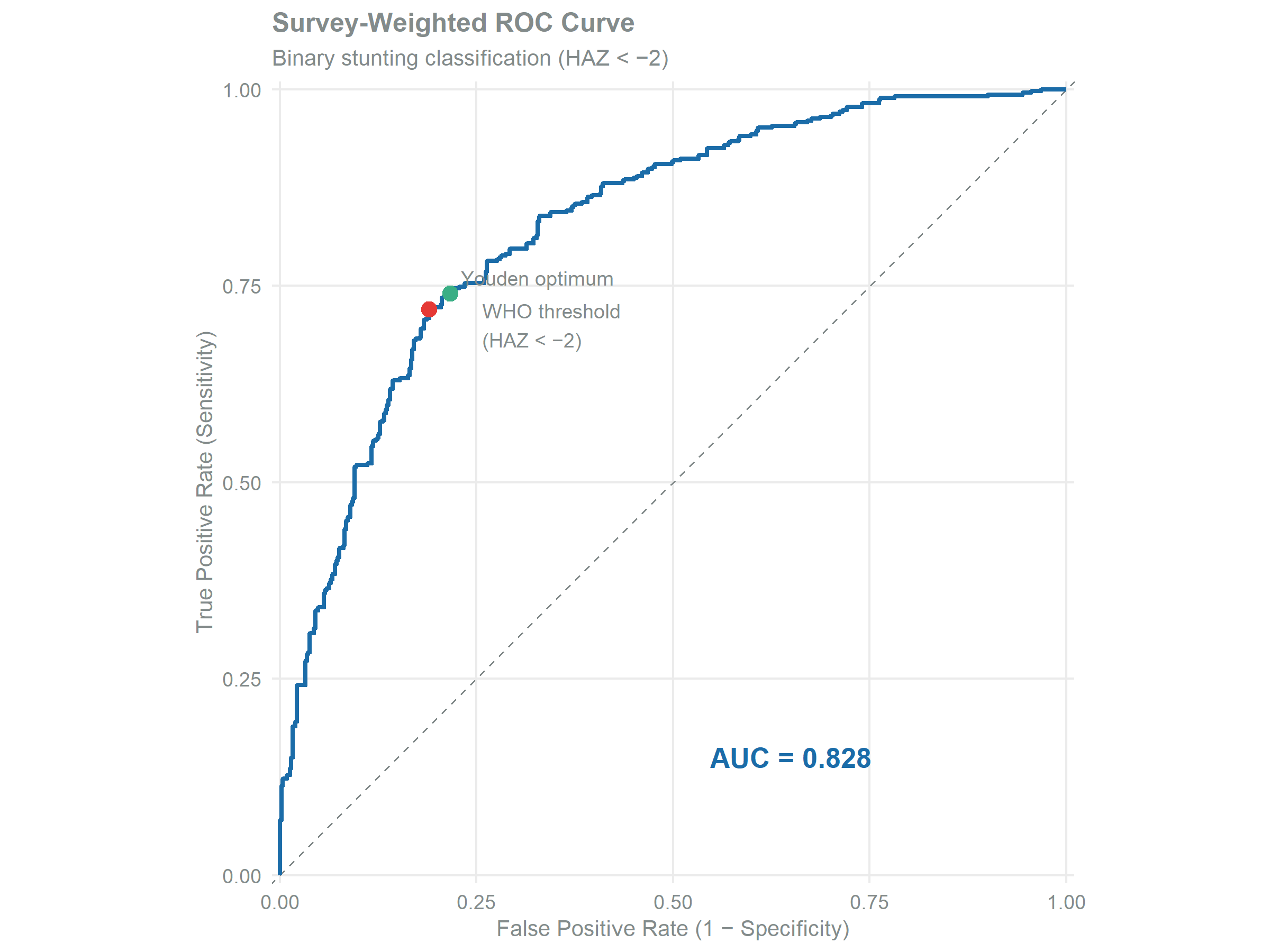
ROC Curve and AUC

Table 8: Survey-weighted AUC and operating point comparison

ROC Analysis Summary. Survey-weighted AUC and operating point comparison
Metric	Value
ROC Analysis Summary
Survey-weighted AUC and operating point comparison
AUC (survey-weighted)	0.828
Sensitivity at WHO threshold	74%
Specificity at WHO threshold	78.3%
Sensitivity at Youden-optimal threshold	72%
Specificity at Youden-optimal threshold	81%
Youden-optimal predicted ZLEN cutoff	-2.073

ROC curve with false positive rate (1 minus specificity) on the x-axis and true positive rate (sensitivity) on the y-axis, plotted against a dashed diagonal chance line. The curve bows above the diagonal toward the top-left corner, giving an area under the curve reported in the annotation, which indicates good discrimination between stunted and non-stunted children. Two marked operating points show the WHO threshold (HAZ below minus 2) and the Youden-optimal cutoff. — Figure 4: Survey-weighted ROC curve for stunting classification

Scope of Evaluation

All metrics in this section are computed in-sample on the training data and represent an upper bound on the model’s true classification performance. The metrics are survey-weighted using pesonino so that they reflect the population of children aged 6–59 months in Guatemala. The WHO threshold (HAZ < −2) is the operationally relevant cutoff for stunting classification; the Youden-optimal threshold is reported as a reference for the maximum classification capacity available from the predicted scores.

Model Performance Summary

Table 9: Final model performance summary

HAZ Continuous Model Performance. Survey-weighted linear regression with polynomial terms
Metric	Value
HAZ Continuous Model Performance
Survey-weighted linear regression with polynomial terms
Model Configuration
Observations Used	751
Model Fit
R²	0.445
RMSE	0.913
MAE	0.706

GAM Effect Model for Impact Simulation

The survey-weighted linear regression provides population-level predictions, but biofortification impact may vary across the nutritional distribution. Children with lower baseline nutrition might benefit more from nutrient improvements than those already well-nourished.

To capture this heterogeneity, we fit a Generalized Additive Model (GAM) that estimates local marginal effects — how much the z-score changes per unit increase in the nutritional index at different points in the distribution — conditional on child age and sex.

Biofortification-Specific Index

Impact simulation uses a nutritional index built from the four nutrients whose intake biofortified maize modifies:

Iron (absorbed)
Zinc (TAZ from Miller equation)
Lysine
Tryptophan

Biofortified varieties raise the lysine and tryptophan content of the grain, and that amino acid profile is what sets the protein quality of a maize-based diet. Representing the mechanism through the two amino acids assigns the change to the quantities that carry it and gives each nutrient a single point of entry into the index.

\[NI_{bio}^{nomaiz} = \frac{1}{4} \times (Fe_{absorbed,z} + Zn_{absorbed,z} + Lys_{z} + Trp_{z})\]

Non-Maize Basis

The index is built exclusively from the non-maize sources of the calibrated block. The full model above uses the six-component nutritional_index; the two are independent objects.

The basis is a question of identification. In these data the observable variation in maize-source nutrients is variation in maize quantity, and maize dependency is a marker of household resources: within the same socioeconomic stratum, a diet more skewed to maize accompanies a lower height-for-age z-score. The non-maize channel carries nutrients that arrive without that marker, and its association with the outcome is positive and of a magnitude consistent with the external evidence.

Quality Protein Maize does not change how much maize a child eats; it changes the nutrient content of the maize already eaten. The increment is therefore treated downstream as additional nutrient arriving in the non-maize pool, which rests on the assumption that a milligram of iron acts the same whatever food carried it. Bioavailability is handled separately through the iron fraction and the Miller model, so that assumption applies to the quantity and not to its absorption.

Two consequences follow. The axis has its own normalization parameters, computed here and exported separately, so that the scripts rebuilding the index from a child’s own non-maize intake work in the units the smooth was estimated in. And the Chispitas contribution sits inside the axis: it was added to non-maize iron and zinc in Chispitas Supplementation, and its departmental equivalent is added to the synthetic population, so the channel is present on both sides by construction.

Scope of the Estimate

The smooth loses statistical significance once socioeconomic covariates enter the specification. The fitted slope is a descriptive dose-response, not an identified causal effect.

GAM Effect Curve

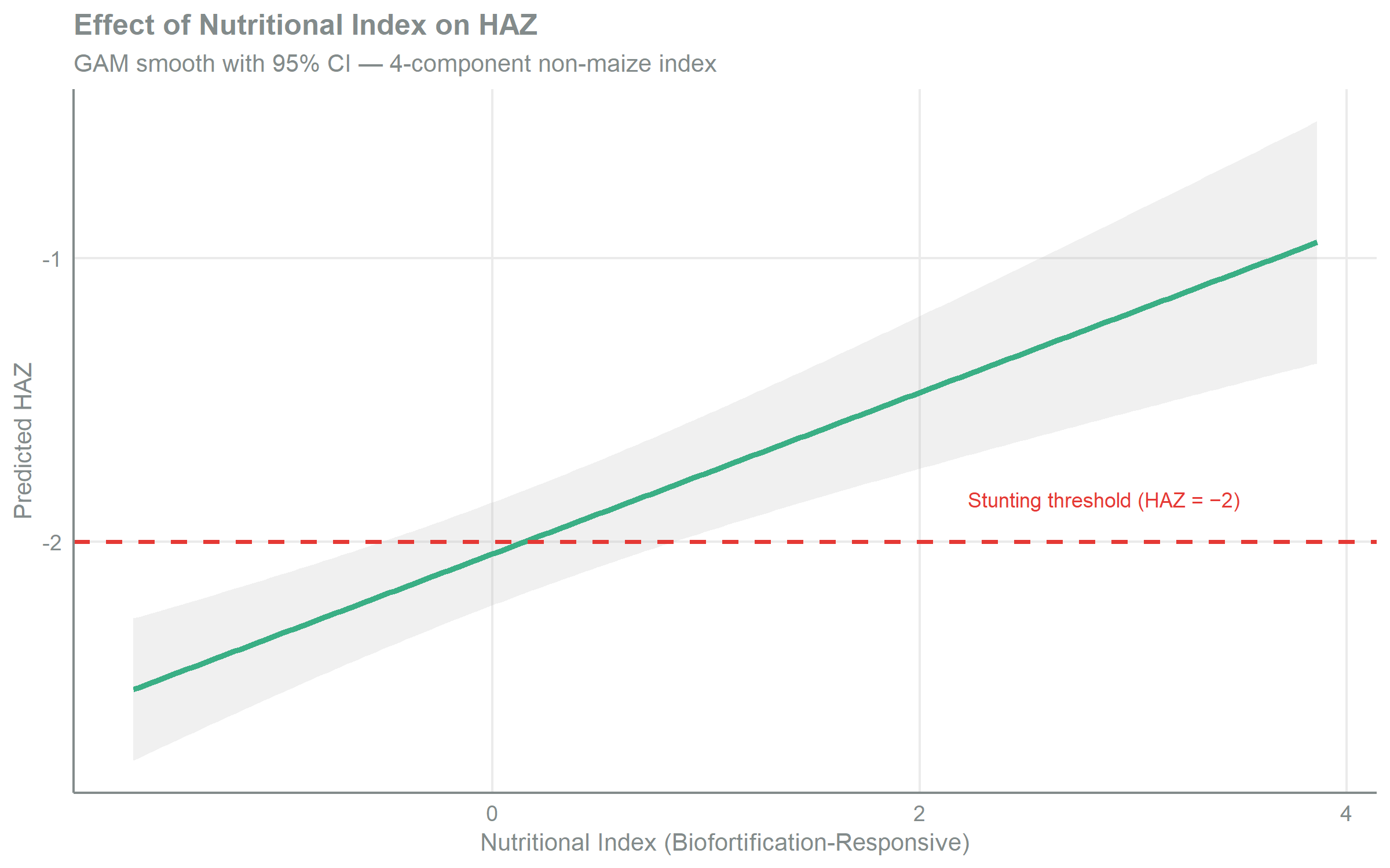
The smooth curve shows how predicted Z-score changes across the nutritional index distribution. The stunting threshold (HAZ = −2) is marked for reference.

Line chart with the biofortification-responsive nutritional index on the x-axis and predicted height-for-age z-score on the y-axis, showing a GAM smooth curve inside a shaded 95% confidence band. The curve rises as the nutritional index increases, so better nutrient adequacy predicts higher z-scores. A dashed horizontal line marks the stunting threshold at HAZ equals minus 2 for reference. — Figure 5: Effect of biofortification-specific nutritional index on HAZ

Marginal Effect Analysis

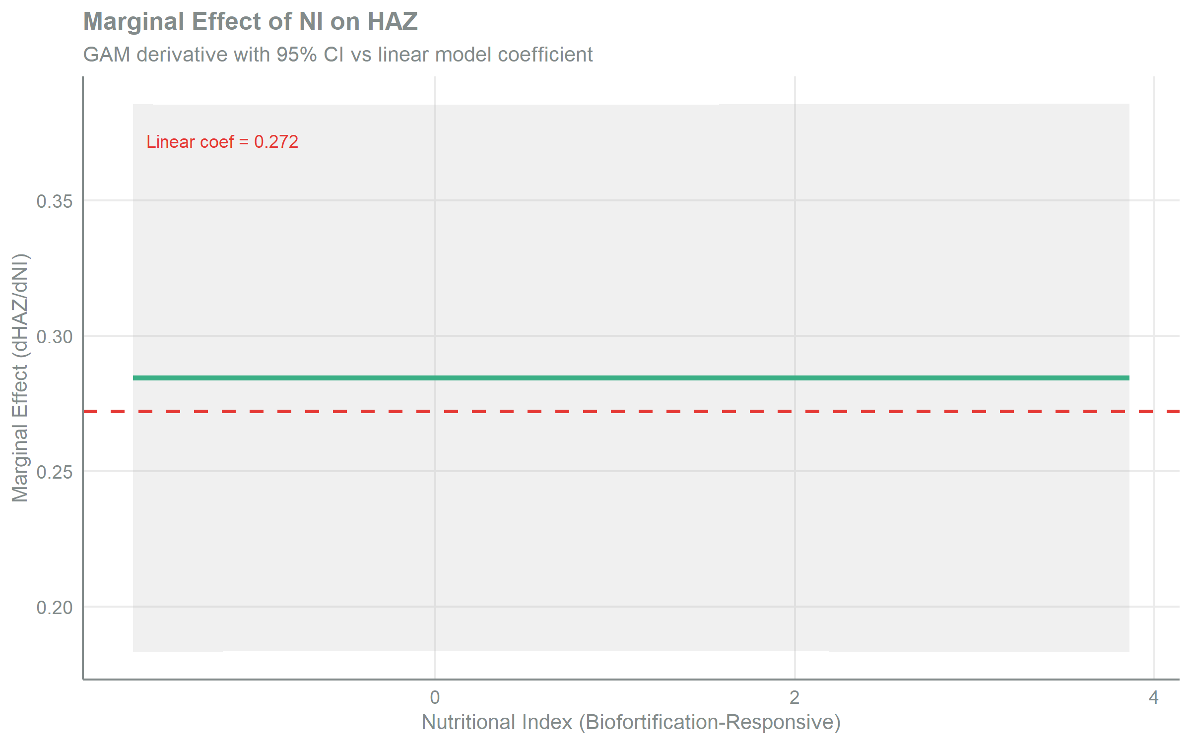
The derivative of the GAM smooth shows how the marginal effect of nutrition on the z-score varies across the distribution. The dashed reference line shows the linear-model coefficient for comparison.

Line chart with the biofortification-responsive nutritional index on the x-axis and the marginal effect (derivative of HAZ with respect to the index) on the y-axis, showing the GAM derivative with a shaded 95% confidence band and a dashed horizontal line at the constant linear-model coefficient. The GAM curve is essentially flat across the whole index range and sits just above the linear coefficient, so the marginal effect estimated by the smooth is close to constant. — Figure 6: Marginal effect of NI on HAZ across the distribution

Shape of the Smooth

On this axis the estimated marginal effect is close to constant: the derivative stays between 0.284 and 0.285 across an index range spanning −1.7 to 3.9, and its ratio to the linear coefficient at the stunted median is 1.04x. The specification admits curvature and the fitted smooth returns little of it, so the GAM and the linear coefficient give nearly the same marginal effect at every point of the distribution.

GAM Model Verification

Table 10: GAM model verification and comparison with linear specification

GAM Model Verification. 4-component non-maize NI (Fe, Zn, lysine, tryptophan) — GAM vs linear
Category	Value
GAM Model Verification
4-component non-maize NI (Fe, Zn, lysine, tryptophan) — GAM vs linear
Impact at Target Population
GAM Marginal Effect at Stunted Median	0.2845
Ratio GAM/Linear at Stunted Median	1.04x
NI Distribution by Stunting Status
Median NI (Stunted Children)	-0.284
Median NI (Non-Stunted Children)	-0.012
Coefficient Comparison
Linear Model Coefficient (NI)	0.2722
GAM Mean Marginal Effect	0.2845
Model Fit
GAM Deviance Explained	6.3%
GAM Effective DF	6.6
The ratio compares the GAM marginal effect at the stunted median against the constant linear coefficient.

Table 11: Complete-case coverage of the GAM variables

GAM Fit Coverage. Observations available for the outcome, the index and the adjustment terms
Variable	Observed	Total	% Complete
GAM Fit Coverage
Observations available for the outcome, the index and the adjustment terms
zlen	751	751	100.0
edad_mes_nino	751	751	100.0
sexo_factor	751	751	100.0
nutritional_index_bio_nomaiz	751	751	100.0

Summary

Model Overview

This module developed a survey-weighted continuous HAZ model with a data-driven formula (43 final terms; 1 predictors dropped by the correlation filter), and a complementary GAM for impact simulation:

Model	Purpose	Key Feature
Survey-weighted linear regression	Population prediction	Data-driven formula with polynomial degrees inferred from univariate GAMs
Binary classification (derived)	Stunting status evaluation	HAZ-thresholded at −2; survey-weighted ROC AUC = 0.828
GAM with biofortification index	Impact simulation	Non-maize index with age and sex adjustment; GAM/linear ratio 1.04x at the stunted median

Key Results

In-sample R²: 0.445 over 751 observations.
Observed vs predicted stunting prevalence (survey-weighted): 44.9% vs 45%.
Classification performance at WHO threshold: sensitivity 74%, specificity 78.3%.
Discrimination: survey-weighted ROC AUC = 0.828.

Application in Impact Simulation

For each child in the synthetic population, the GAM-based simulation:

Calculates the new non-maize index post-biofortification: \(NI_{new} = NI_{baseline} + \Delta NI\)
Evaluates the GAM at both index values, holding age and sex at their observed values: \(f(NI_{baseline})\) and \(f(NI_{new})\)
Takes the z-score change as the difference of the two fitted values: \(\Delta HAZ = f(NI_{new}) - f(NI_{baseline})\)
Classifies new stunting status: stunted if \((HAZ_{baseline} + \Delta HAZ) < -2\)

Taking the difference of fitted values, rather than a first-order term, lets the estimate follow the curvature of the smooth across the whole interval the index traverses.

Limitations

Impact simulation scope — The GAM is intended for aggregate impact estimation, not individual-level HAZ prediction.
Extrapolation uncertainty — Confidence intervals widen at distribution extremes where data is sparse.
Proportionality assumption — Impact estimates assume biofortification affects index components proportionally to established biofortification factors.
In-sample classification metrics — Sensitivity, specificity, and AUC are computed on the training data and represent an upper bound on out-of-sample performance.