Transfer Height to ENCOVI

Module 5: Meta-analysis

Why Transfer Height to ENCOVI?

ENCOVI 2023 does not include anthropometric measurements for children. To estimate the stunting impact of biofortified maize, we need individual-level height predictions that can be converted to height-for-age z-scores (HAZ). This module bridges that gap through a four-stage pipeline:

GAM prediction — Apply the trained height model to ENCOVI 2023 children using their socioeconomic profiles
Quantile mapping — Calibrate predicted heights against Guatemala-specific reference distributions derived from ENSMI stunting prevalence and WHO growth standards
HAZ calculation — Convert calibrated heights to height-for-age z-scores and classify stunting status
Weight calibration — Adjust survey weights to match ENSMI 2014-2015 departmental stunting prevalence

Data Sources

Three external inputs are required: the trained GAM model with its transformation objects, from the two preceding steps of this module; the WHO LMS growth reference parameters; and the ENSMI 2014-2015 departmental stunting targets.

Table 1: WHO LMS reference table summary

WHO LMS Reference Parameters. Length/height-for-age by sex and age in months
Sex	Age Points	Age Range	Median (SD0) Height Range
WHO LMS Reference Parameters
Length/height-for-age by sex and age in months
Hombre	61	0-60 months	49.9-110 cm
Mujer	61	0-60 months	49.1-109.4 cm

Target Population and Exclusions

Population Identification

Table 2: ENCOVI 2023 children 6-59 months target population

Target Population Identification. ENCOVI 2023 children aged 6-59 months, on the age assigned in Module 1
Metric	Value
Target Population Identification
ENCOVI 2023 children aged 6-59 months, on the age assigned in Module 1
Total individuals in ENCOVI 2023	46,017
Children aged 6-59 months	4,233
Weighted population (6-59 months)	1,606,843

Dietary Record Completeness

The analytical cohort is restricted to children whose household reports a complete dietary record: the food consumption module supplies their source-specific nutrient intake and the plant-source share of that intake. Both quantities are required downstream by the bioavailability, inadequacy and nutrient-profile calculations, and the twelve intake variables are recorded together, so completeness is required on the full set rather than on any single component.

The restriction is applied before weight calibration, so the departmental stunting prevalence targets are calibrated over the population that reaches the analysis. It removes 168 of the 4,233 children aged 6-59 months.

Table 3: Records excluded for an incomplete dietary record

Dietary Record Completeness. Cohort restricted to children with nutrient intake and plant-source share
Metric	Value
Dietary Record Completeness
Cohort restricted to children with nutrient intake and plant-source share
Children 6-59 months (pre-exclusion)	4,233
Excluded: incomplete dietary record	168
Children 6-59 months (post-exclusion)	4,065
Weighted population (post-exclusion)	1,522,562

Predictor Harmonization and Imputation

ENCOVI variables are recoded to match the coding structure used in SIVESNU, and the normalization objects fitted there are applied to the continuous predictors, so both surveys enter the model on the same scale. Missing values are imputed via Random Forest using the impute_rf_parallel() utility function, which wraps missRanger::missRanger() with a multi-threaded ranger engine.

Table 4: Missing values in GAM predictor variables

Missing Values in Predictor Variables. ENCOVI 2023 children 6-59 months
Variable	N_Missing	Pct_Missing
Missing Values in Predictor Variables
ENCOVI 2023 children 6-59 months
tipo_sanitario	237	5.8%
recoleccion_basura	224	5.5%
grado_estudios_hogar	4	0.1%

Where the Missingness Sits

3 predictors carry missing values in the analytical cohort. Two of them account for almost all of it: tipo_sanitario at 5.8% of records and recoleccion_basura at 5.5%, both service-provision indicators. grado_estudios_hogar is missing for 4 records. Random Forest imputation fills these values from the rest of the predictor set.

Height Prediction

The trained GAM model is applied to generate height predictions for each ENCOVI child based on their socioeconomic profile.

Table 5: Predicted height summary by age group

Predicted Height Distribution by Age Group. ENCOVI 2023 children 6-59 months — GAM predictions
Age Group	N	Mean (cm)	SD (cm)	Min (cm)	Max (cm)
Predicted Height Distribution by Age Group
ENCOVI 2023 children 6-59 months — GAM predictions
6-11m	421	65.8	2.6	59.2	72.4
12-23m	844	74.1	3.3	64.7	83.7
24-35m	902	82.7	3.0	74.6	92.6
36-47m	865	90.3	2.9	83.0	98.9
48-59m	1033	97.0	2.6	89.8	104.6

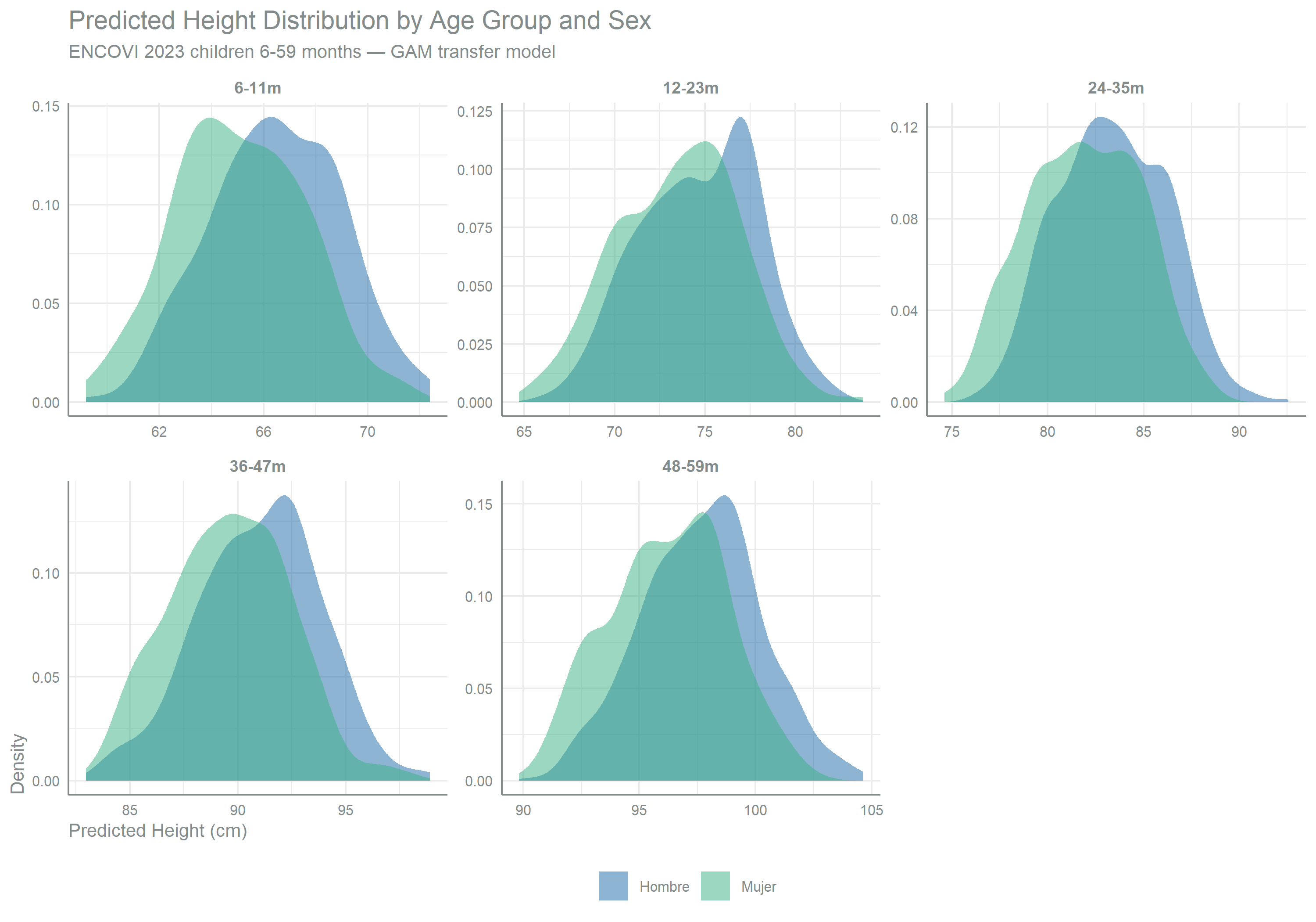
Faceted density plot with one panel per age group, showing GAM-predicted height in centimetres on the x-axis and density on the y-axis, with separate overlaid curves for boys and girls. Within each panel the curves are narrow and concentrated, illustrating that predictions capture only the conditional mean and so compress variance relative to true population spread, a compression corrected by the later quantile-mapping step. — Figure 1: Predicted height distribution by age group and sex

Prediction Variance

GAM predictions capture the conditional mean of height given socioeconomic predictors, producing narrower distributions than expected population variability. This variance compression is corrected by quantile mapping in the next step.

Quantile Mapping Calibration

Stratification

Children are partitioned into 18 strata (9 six-month age bands × 2 sexes) for quantile mapping. Each stratum receives its own reference distribution parameters.

Table 6: Sample size per age-sex stratum

Sample Size per Age-Sex Stratum. ENCOVI 2023 children 6-59 months — 18 strata for quantile mapping
Age Band	Hombre		Mujer
Sample Size per Age-Sex Stratum
ENCOVI 2023 children 6-59 months — 18 strata for quantile mapping
Age Band	N	Weighted N	N	Weighted N
6-11	223	91,905	198	79,185
12-17	208	83,785	201	73,497
18-23	221	81,831	214	73,155
24-29	222	93,460	209	83,731
30-35	250	86,713	221	74,831
36-41	218	77,935	204	78,913
42-47	227	77,152	216	74,556
48-53	257	100,588	245	92,046
54-59	270	103,527	261	95,752

Guatemala-Specific Reference Distributions

For each stratum, the expected height distribution is derived from WHO LMS parameters and ENSMI national stunting prevalence (46.5%). The Guatemala-specific mean (mu) is solved from the equation P(height < threshold) = p_stunting, and sigma is set to the WHO reference SD.

Table 7: Guatemala-specific reference distribution parameters by stratum

Guatemala-Specific Reference Distributions. Derived from WHO LMS parameters and ENSMI 2014-2015 stunting prevalence (46.5%)
Age Band	Sex	Midpoint Age	WHO Median (M)	Stunting Threshold (cm)	Guatemala mu (cm)	Guatemala sigma (cm)
Guatemala-Specific Reference Distributions
Derived from WHO LMS parameters and ENSMI 2014-2015 stunting prevalence (46.5%)
6-11	Hombre	8	70.60	66.19	66.38	2.21
6-11	Mujer	8	68.75	64.02	64.23	2.36
12-17	Hombre	14	78.05	73.10	73.31	2.48
12-17	Mujer	14	76.38	71.01	71.25	2.68
18-23	Hombre	20	84.20	78.57	78.82	2.81
18-23	Mujer	20	82.70	76.68	76.94	3.01
24-29	Hombre	26	88.81	82.46	82.73	3.18
24-29	Mujer	26	87.45	80.79	81.08	3.33
30-35	Hombre	32	93.38	86.35	86.66	3.51
30-35	Mujer	32	92.19	84.94	85.26	3.63
36-41	Hombre	38	97.37	89.78	90.11	3.80
36-41	Mujer	38	96.42	88.63	88.97	3.90
42-47	Hombre	44	101.04	92.95	93.31	4.04
42-47	Mujer	44	100.31	92.01	92.37	4.15
48-53	Hombre	50	104.45	95.91	96.29	4.27
48-53	Mujer	50	103.90	95.13	95.52	4.38
54-59	Hombre	56	107.77	98.79	99.19	4.49
54-59	Mujer	56	107.28	98.06	98.46	4.61
mu_guatemala = height_threshold - sigma × Φ⁻¹(p_stunting) sigma_guatemala = M × S (WHO reference SD)

Quantile Mapping Rationale

GAM predictions compress variance relative to the true population. Normal quantile mapping corrects this by transforming each predicted height through the source CDF and back through the Guatemala-specific inverse CDF, preserving rank order while expanding the distribution to match the expected population variability.

Quantile Mapping Application and Diagnostics

Table 8: Height distribution before and after quantile mapping

Height Distribution: Before vs After Quantile Mapping. Normal QM within 6-month age bands by sex — Guatemala-specific reference
Stage	Mean (cm)	SD (cm)	Median (cm)	Min (cm)	Max (cm)
Height Distribution: Before vs After Quantile Mapping
Normal QM within 6-month age bands by sex — Guatemala-specific reference
Before QM (predicted)	84.40	10.70	85.38	59.2	104.6
After QM (calibrated)	85.33	11.23	86.71	58.6	112.6

Table 9: Quantile mapping effect by age-sex stratum

Quantile Mapping Effect by Stratum. Comparison of predicted, calibrated, and reference parameters
Age Band	Sex	N	Pred Mean	Cal Mean	Ref Mean	Δ Mean	Pred SD	Cal SD
Quantile Mapping Effect by Stratum
Comparison of predicted, calibrated, and reference parameters
6-11	Hombre	223	66.5	66.3	66.4	-0.2	2.48	2.23
6-11	Mujer	198	65.1	64.4	64.2	-0.7	2.48	2.44
12-17	Hombre	208	72.3	73.4	73.3	1.1	2.42	2.69
12-17	Mujer	201	71.0	71.4	71.2	0.4	2.48	2.72
18-23	Hombre	221	76.9	78.8	78.8	1.9	2.06	2.70
18-23	Mujer	214	75.8	77.1	76.9	1.3	2.22	3.04
24-29	Hombre	222	81.3	82.8	82.7	1.5	1.95	3.32
24-29	Mujer	209	79.7	81.1	81.1	1.4	2.02	3.46
30-35	Hombre	250	85.2	86.9	86.7	1.7	2.16	3.47
30-35	Mujer	221	84.0	85.8	85.3	1.8	1.97	3.70
36-41	Hombre	218	89.1	90.1	90.1	1.0	2.25	3.84
36-41	Mujer	204	87.7	88.9	89.0	1.2	2.17	4.07
42-47	Hombre	227	92.8	93.6	93.3	0.8	1.98	4.04
42-47	Mujer	216	91.4	92.2	92.4	0.8	2.05	4.15
48-53	Hombre	257	96.2	96.3	96.3	0.1	2.17	4.18
48-53	Mujer	245	94.5	95.9	95.5	1.4	2.06	4.64
54-59	Hombre	270	99.1	99.4	99.2	0.3	1.95	4.67
54-59	Mujer	261	97.8	98.7	98.5	0.9	1.85	4.82

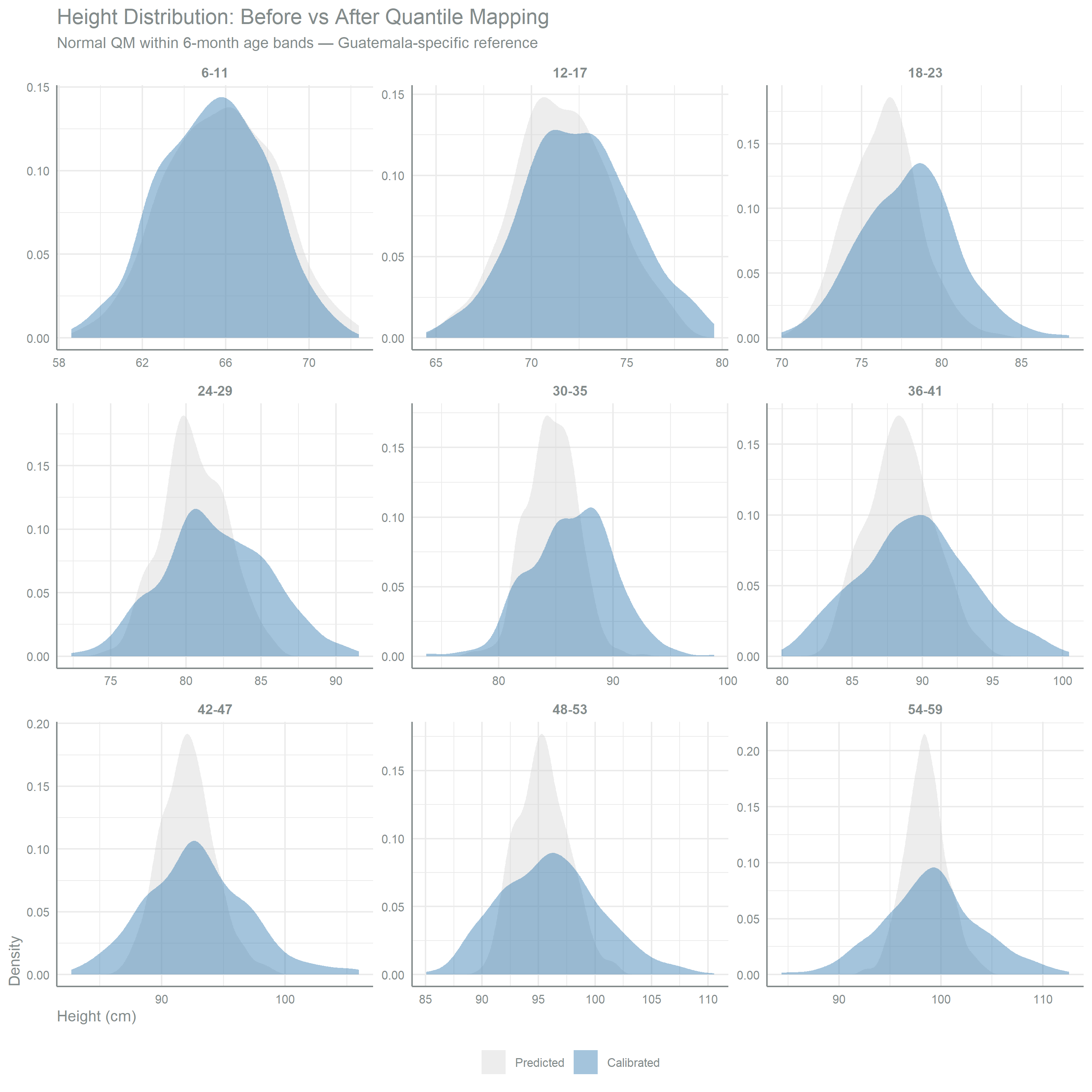
Faceted density plot with one panel per six-month age band, showing height in centimetres on the x-axis and density on the y-axis. Each panel overlays two curves: the narrow predicted distribution before calibration and the wider calibrated distribution after quantile mapping. From the 12-month band onward the calibrated curve is visibly wider than the predicted one; in the 6-11 month band the two curves nearly coincide. — Figure 2: Height distribution before and after quantile mapping by age band

Quantile Mapping Effect

Calibration moves the height distributions onto the Guatemala-specific reference means and widens their spread, taking the pooled SD from 10.70 cm to 11.23 cm. Table 9 reports the calibrated mean against the reference mean for each of the 18 strata.

HAZ Calculation and Stunting Classification

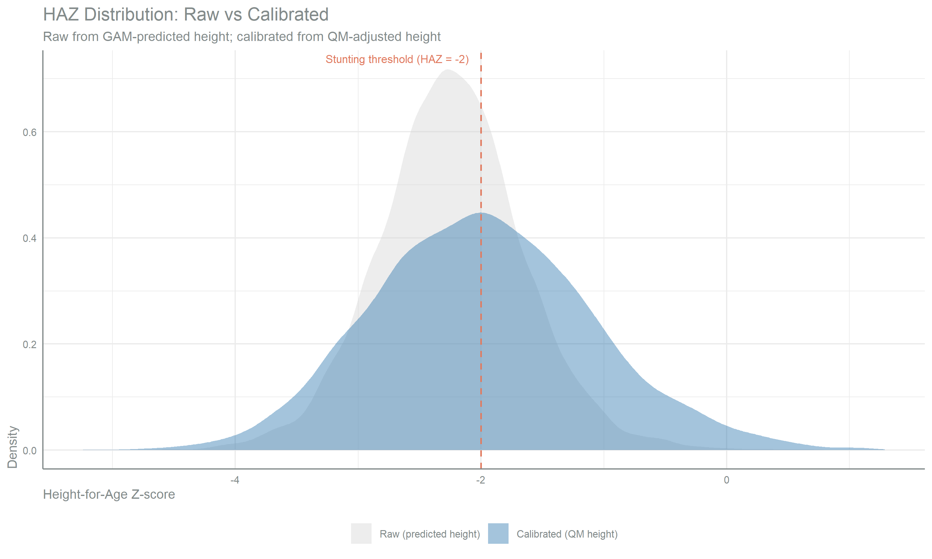
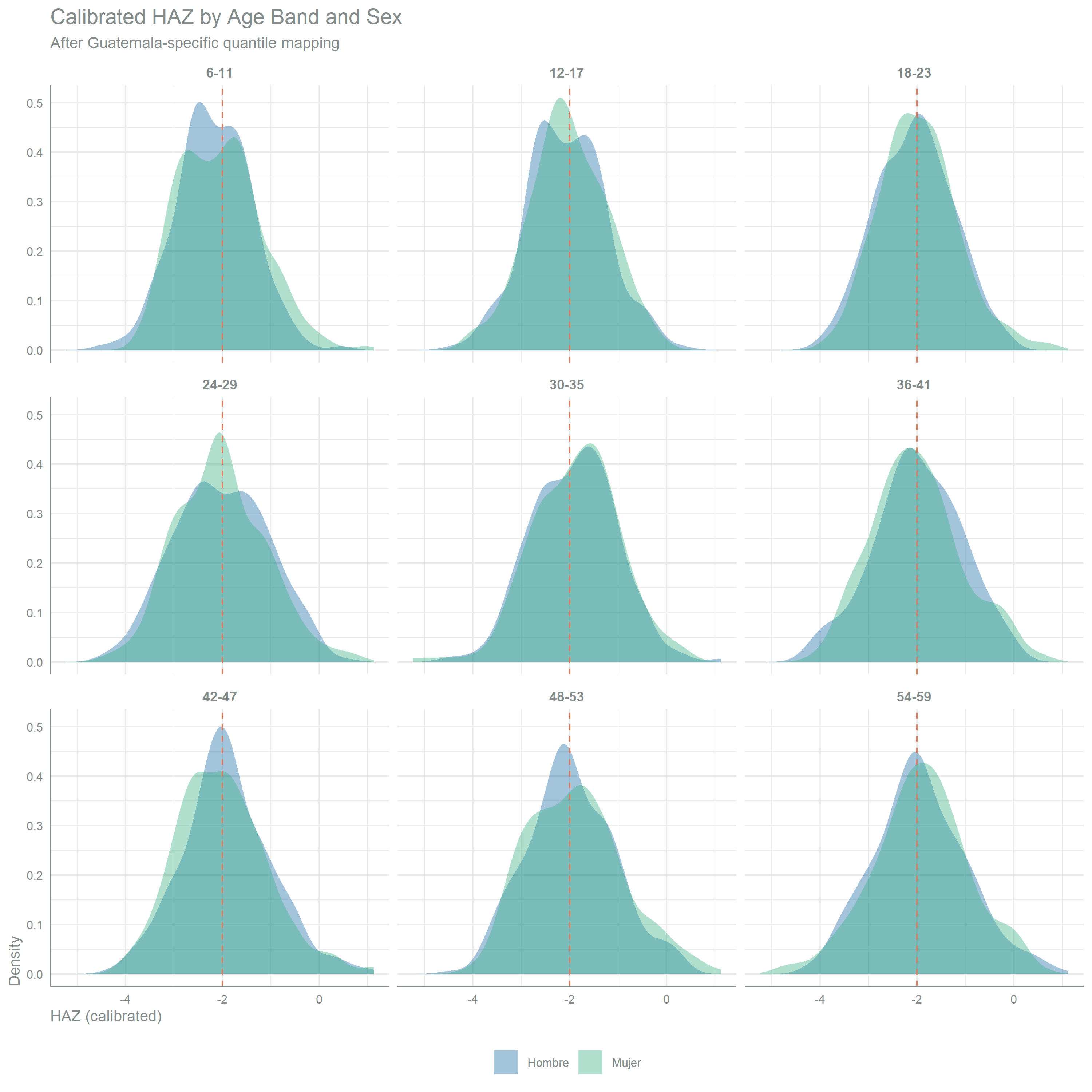
Calibrated heights are converted to height-for-age z-scores using the WHO LMS formula. For length/height-for-age, L = 1 across all ages, simplifying to HAZ = (height − M) / (M × S), where M is the median height-for-age from the WHO reference and S is the coefficient of variation. Stunting is classified as HAZ < −2.

Table 10: HAZ distribution summary: raw vs calibrated

HAZ Distribution: Raw vs Calibrated. Raw HAZ from GAM-predicted height; calibrated HAZ from QM-adjusted height
Stage	Mean	SD	Median	Stunting %	Range
HAZ Distribution: Raw vs Calibrated
Raw HAZ from GAM-predicted height; calibrated HAZ from QM-adjusted height
Raw (from predicted height)	-2.241	0.597	-2.249	67.2	[-4.55, 1.29]
Calibrated (from QM height)	-1.984	0.893	-2.009	50.5	[-5.24, 1.13]

Departmental HAZ Before Weight Calibration

Table 11: Calibrated HAZ and stunting prevalence by department

Departmental HAZ and Stunting Prevalence (Pre-Calibration). Survey-weighted estimates before weight calibration — comparison with ENSMI targets
Department	N	Mean HAZ	SD HAZ	Stunting %	ENSMI Target %	Diff (pp)¹
Departmental HAZ and Stunting Prevalence (Pre-Calibration)
Survey-weighted estimates before weight calibration — comparison with ENSMI targets
Alta Verapaz	247	−2.056	0.670	57.8	50.0	7.8
Baja Verapaz	203	−1.872	0.824	47.2	50.2	−3.0
Chimaltenango	204	−2.428	0.908	67.4	56.5	10.9
Chiquimula	136	−1.499	0.946	35.7	55.6	−19.9
El Progreso	138	−2.329	0.878	64.0	29.1	34.9
Escuintla	208	−2.168	0.841	54.6	26.9	27.7
Guatemala	173	−2.044	0.788	49.2	25.3	23.9
Huehuetenango	207	−2.185	0.968	60.9	67.7	−6.8
Izabal	191	−1.631	0.908	37.2	26.4	10.8
Jalapa	196	−1.562	0.891	28.7	53.8	−25.1
Jutiapa	173	−1.028	0.900	11.8	35.7	−23.9
Petén	200	−1.725	0.783	32.8	36.1	−3.3
Quetzaltenango	174	−1.854	0.801	43.5	48.8	−5.3
Quiché	274	−2.174	0.718	64.5	68.7	−4.2
Retalhuleu	138	−2.164	0.742	59.6	34.2	25.4
Sacatepéquez	168	−2.012	0.766	47.7	42.4	5.3
San Marcos	204	−2.348	0.800	71.8	54.8	17.0
Santa Rosa	117	−2.256	0.936	59.5	33.6	25.9
Sololá	146	−1.985	0.761	51.5	65.6	−14.1
Suchitepéquez	223	−1.958	0.847	46.6	39.6	7.0
Totonicapán	194	−2.386	0.755	69.4	70.0	−0.6
Zacapa	151	−1.495	0.910	26.4	40.0	−13.6
¹ Red: > 10 pp deviation. Yellow: 5-10 pp deviation. Weight calibration corrects these differences.

Pre-Calibration Deviations

Before weight calibration, 13 of 22 departments sit more than 10 percentage points away from their ENSMI stunting target and a further 5 between 5 and 10, with the widest gap at 34.9 pp. The gaps run in both directions, which places them in the geographic distribution of the model’s predictions rather than in a uniform level shift. The weight calibration step closes them.

HAZ Distribution Visualization

Density plot of height-for-age z-score on the x-axis against density on the y-axis, overlaying two curves: raw HAZ from GAM-predicted height and calibrated HAZ from quantile-mapped height. A dashed vertical line marks the stunting threshold at HAZ equal to minus 2. The calibrated curve is wider than the compressed raw curve and its centre sits slightly higher, so it leaves less mass below the threshold and moves closer to Guatemala's reference prevalence. — Figure 3: HAZ distribution: raw vs calibrated

Faceted density plot with one panel per six-month age band, showing calibrated height-for-age z-score on the x-axis and density on the y-axis, with separate overlaid curves for boys and girls and a dashed vertical line at the stunting threshold of HAZ equal to minus 2. Across panels the distributions for both sexes are broadly similar in location and spread, indicating consistent calibrated HAZ across age bands and sexes. — Figure 4: Calibrated HAZ distribution by age band and sex

Weight Calibration

Survey weights are adjusted so that weighted stunting prevalence matches ENSMI 2014-2015 departmental targets exactly. This corrects residual discrepancies between the model-implied stunting rates and official estimates, while preserving total weighted population per department.

Calibration Diagnostics

Table 12: Weight calibration diagnostics

Survey Weight Calibration Diagnostics. Calibrated to ENSMI 2014-2015 departmental stunting prevalence
Metric	Value
Survey Weight Calibration Diagnostics
Calibrated to ENSMI 2014-2015 departmental stunting prevalence
Weight CV (initial)	73.55%
Weight CV (calibrated)	85.36%
Design Effect (DEFF)	1.729
Adjustment ratio range	[0.455, 3.017]
Ratios < 0.3 (extreme low)	0
Ratios > 3.0 (extreme high)	25
Mean adjustment ratio	1.005

Departmental Stunting Validation

Table 13: Stunting prevalence by department: calibrated vs ENSMI targets

Departmental Stunting Prevalence Validation. Calibrated weighted prevalence vs ENSMI 2014-2015 targets
Department	N	ENSMI Target (%)	Calibrated (%)	Diff (pp)¹
Departmental Stunting Prevalence Validation
Calibrated weighted prevalence vs ENSMI 2014-2015 targets
Alta Verapaz	247	50.0	50.0	0.00
Baja Verapaz	203	50.2	50.2	0.00
Chimaltenango	204	56.5	56.5	0.00
Chiquimula	136	55.6	55.6	0.00
El Progreso	138	29.1	29.1	0.00
Escuintla	208	26.9	26.9	0.00
Guatemala	173	25.3	25.3	0.00
Huehuetenango	207	67.7	67.7	0.00
Izabal	191	26.4	26.4	0.00
Jalapa	196	53.8	53.8	0.00
Jutiapa	173	35.7	35.7	0.00
Petén	200	36.1	36.1	0.00
Quetzaltenango	174	48.8	48.8	0.00
Quiché	274	68.7	68.7	0.00
Retalhuleu	138	34.2	34.2	0.00
Sacatepéquez	168	42.4	42.4	0.00
San Marcos	204	54.8	54.8	0.00
Santa Rosa	117	33.6	33.6	0.00
Sololá	146	65.6	65.6	0.00
Suchitepéquez	223	39.6	39.6	0.00
Totonicapán	194	70.0	70.0	0.00
Zacapa	151	40.0	40.0	0.00
¹ Red: departments with > 1 pp deviation from target.

What the Calibration Costs

The 22 departments reach their ENSMI stunting target to 0.00 pp. The mean adjustment ratio is 1.005, so the total weight is preserved, but the adjustment is not evenly distributed: individual ratios span [0.455, 3.017], and 25 units sit above 3.0.

The dispersion of the weights therefore rises. Their coefficient of variation moves from 73.55% to 85.36%, and the design effect stands at 1.729, which means the calibrated sample carries the precision of one about 1.73 times smaller. Departmental alignment is obtained at that price.

National Indicators

Table 14: National stunting and HAZ indicators after weight calibration

National Stunting and HAZ Indicators. ENCOVI 2023 children 6-59 months — after departmental weight calibration to ENSMI 2014-2015
Metric	Value
National Stunting and HAZ Indicators
ENCOVI 2023 children 6-59 months — after departmental weight calibration to ENSMI 2014-2015
N children (6-59 months)	4,065
Weighted population	1,522,562
Stunting prevalence (HAZ < -2)	48.58%
ENSMI 2014-2015 official stunting prevalence	46.5%
Stunting deviation from ENSMI	2.08 pp
Mean HAZ (weighted)	-1.976
ENSMI 2014-2015 official mean HAZ	-1.9
HAZ deviation from ENSMI	-0.076
SD HAZ (weighted)	0.85
Median HAZ (unweighted)	-2.009
HAZ range	[-5.24, 1.13]

National Indicators

After calibration the weighted stunting prevalence is 48.58% against the ENSMI national figure of 46.5%, a gap of 2.08 pp. The calibration targets are departmental, so the national aggregate also carries the composition of ENCOVI’s sample across departments, which need not match the composition behind the ENSMI national figure. The weighted mean HAZ is -1.976 against the official -1.9, a difference of -0.076.

Final Validation Summary

A final validation pass checks completeness of the output dataset and verifies that the calibration procedure achieves its targets at the departmental level.

Table 15: Final validation summary

Final Validation Summary. Height transfer, quantile mapping, and weight adjustment
Check	Value	Status
Final Validation Summary
Height transfer, quantile mapping, and weight adjustment
Total children 6-59 months	4065	—
Children with calibrated height	4065	PASS
Children with HAZ	4065	PASS
Children with stunting classification	4065	PASS
Children with calibrated weights	4065	PASS
Missing calibrated height	0	PASS
Missing HAZ	0	PASS
Missing stunting (hfa)	0	PASS
Missing calibrated weights	0	PASS
HAZ out of [-6, 6]	0	PASS
Negative calibrated weights	0	PASS
Departments with ENSMI match (0.00 pp)	22	PASS

Summary

Key Findings

Height prediction: The GAM transfer model produces a height for each of 4,065 ENCOVI 2023 children aged 6-59 months from their socioeconomic profile.
Quantile mapping: Normal quantile mapping within 18 age-sex strata widens the predicted height distribution from an SD of 10.70 cm to 11.23 cm and aligns each stratum with its Guatemala-specific reference parameters.
HAZ calculation: Calibrated heights give a weighted national stunting prevalence of 48.58% and a mean HAZ of -1.976, 2.08 pp and -0.076 from the ENSMI 2014-2015 official figures.
Weight calibration: The 22 departments reach their ENSMI stunting target to 0.00 pp, with the weight coefficient of variation moving from 73.55% to 85.36%.

Limitations

Model-based heights — Height values are predicted from socioeconomic proxies rather than measured, so the estimates hold at the level of the distribution and not of the individual child.
ENSMI temporal gap — Calibration targets come from ENSMI 2014-2015 and the ENCOVI data are from 2023, so any change in stunting between the two collection periods is absorbed into the calibration.
Quantile mapping assumes normality — The normal quantile mapping treats height as Gaussian within each age-sex stratum, which bounds how well the tails of the calibrated distribution are reproduced.
Weight dispersion — Calibration raises the weight coefficient of variation from 73.55% to 85.36% and leaves 25 units with an adjustment ratio above 3.0, which widens the sampling variance of the weighted estimates.

Application

This dataset — containing predicted height, calibrated HAZ, stunting classification, and calibrated survey weights for 4,065 children — feeds the bioavailability and inadequacy calculations and the QPM stunting impact estimation.