| Distribution Fit Comparison | ||||||
| Goodness-of-fit statistics for Gamma, Lognormal, and Exponential distributions | ||||||
| Distribution | Log-Likelihood |
Information Criteria
|
Goodness-of-Fit Statistics
|
|||
|---|---|---|---|---|---|---|
| AIC | BIC | Kolmogorov-Smirnov | Cramer-von Mises | Anderson-Darling | ||
| Gamma | −130,103.2506 | 260,210.5012 | 260,227.6774 | 0.0617 | 51.2549 | 274.8423 |
| Lognormal | −130,445.5698 | 260,895.1396 | 260,912.3158 | 0.0301 | 11.9193 | 103.4848 |
| Exponential | −131,268.8361 | 262,539.6723 | 262,548.2604 | 0.1150 | 207.7700 | 1,117.2492 |
Transfer Model: Zinc Intake
Module 3: Transfer Models
Why Model Zinc?
Zinc is essential for immune function and growth, and zinc deficiency is associated with stunting in children. In Guatemala, maize provides a substantial share of dietary zinc (see Daily Nutrient Intake by Source in Module 1) — even higher than for iron. By modeling zinc intake from maize and non-maize sources separately, we can:
- Simulate biofortification scenarios — Predict how higher-content maize varieties would change total zinc intake
- Preserve baseline non-maize intake — Keep other dietary sources constant when modeling interventions
- Locate the modifiable fraction — Identify where the maize-derived share of zinc intake is largest
Modeling Approach
We use survey-weighted gamma regression because zinc intake data is:
- Positive and continuous — People consume some amount of zinc daily
- Right-skewed — Most people have moderate intake, few have very high intake
- Population-representative — Survey weights carry the estimates to the national level
The models predict zinc intake based on demographic and socioeconomic characteristics that are available in both ENCOVI (training data) and SIVESNU (application target).
Data Preparation
Source Data
We use the cleaned ENCOVI dataset from the previous preparation step, containing individuals with complete predictor variables and nutrient intake estimates.
Handling Extreme Values
Gamma regression requires positive values and is sensitive to extreme outliers. We apply conservative outlier detection:
TipOutlier Threshold
Upper outliers identified as values exceeding P95 + 1.5×IQR (i.e., 95th percentile plus 1.5 times the interquartile range). The threshold suits micronutrients:
- Micronutrient intake distributions are markedly right-skewed
- Biologically plausible high values arise from consumption of micronutrient-dense or fortified foods
- Retaining the upper tail supports model generalizability to populations with varied dietary patterns
Survey Design
All models incorporate ENCOVI’s complex survey design (clustering and expansion weights), which places the estimates at the population level.
Modeling Zinc Intake from Maize
Distribution Selection
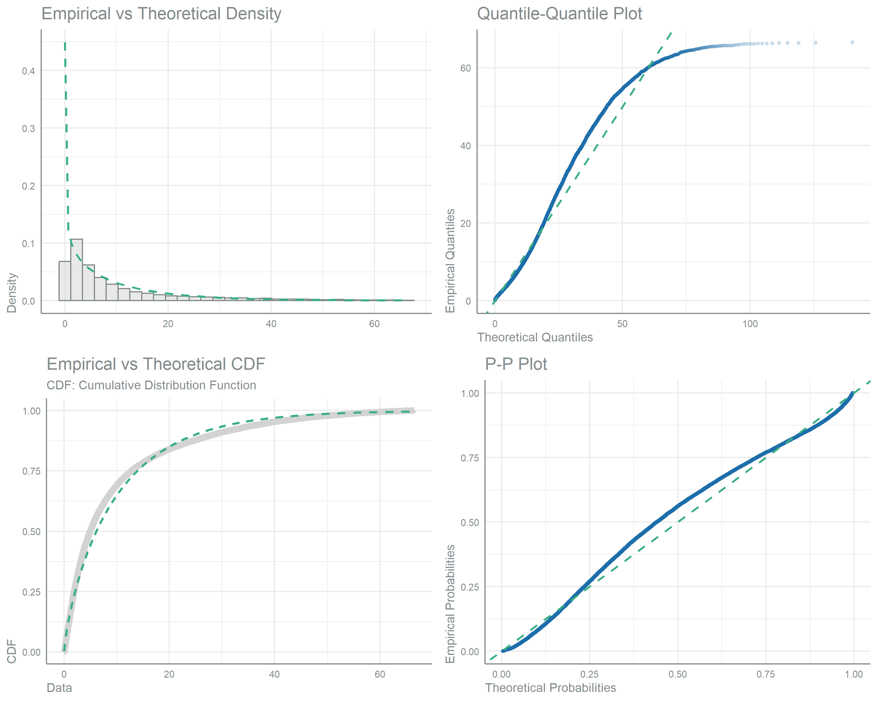
Before modeling, we assess which statistical distribution best fits the zinc intake data. Three candidate distributions are compared:
ImportantDistribution Selection
Gamma distribution provides the best fit based on:
- Lowest AIC/BIC (information criteria)
- Highest Log-Likelihood
Gamma regression with log link is appropriate for positive, right-skewed continuous outcomes.
Full Model
We first train a model including all 20 candidate predictors to identify which variables significantly predict zinc intake from maize.
| Zinc Intake from Maize (Full Model) - Model Coefficients | ||||
| Survey-weighted gamma regression with log link | ||||
| Term | Estimate | Std. Error | t-statistic | p-value |
|---|---|---|---|---|
| (Intercept) | 1.0732 | 0.2003 | 5.3571 | <0.0001 |
| parentescoEsposo(a) o compañero(a) | 0.1486 | 0.0848 | 1.7520 | 0.0800 |
| parentescoHermano(a) | 0.2719 | 0.1482 | 1.8343 | 0.0668 |
| parentescoHijo(a) | 0.3803 | 0.0777 | 4.8935 | <0.0001 |
| parentescoJefe del hogar | 0.1644 | 0.0816 | 2.0154 | 0.0441 |
| parentescoNieto(a) | 0.2715 | 0.0880 | 3.0848 | 0.0021 |
| parentescoOtro no pariente | 0.3925 | 0.4109 | 0.9552 | 0.3396 |
| parentescoOtro pariente | 0.3064 | 0.1246 | 2.4595 | 0.0140 |
| parentescoPadre o madre | 0.3368 | 0.0896 | 3.7604 | 0.0002 |
| parentescoSuegro(a) | 0.3453 | 0.1405 | 2.4569 | 0.0141 |
| parentescoYerno o nuera | 0.3299 | 0.1433 | 2.3026 | 0.0215 |
| sexoMujer | −0.1269 | 0.0190 | −6.6747 | <0.0001 |
| poly(edad, 2)1 | 41.5762 | 4.4335 | 9.3777 | <0.0001 |
| poly(edad, 2)2 | −31.9618 | 2.0630 | −15.4927 | <0.0001 |
| departamentoEl Progreso | 0.2687 | 0.1269 | 2.1171 | 0.0344 |
| departamentoSacatepéquez | 0.2788 | 0.1041 | 2.6788 | 0.0075 |
| departamentoChimaltenango | 0.4921 | 0.1021 | 4.8179 | <0.0001 |
| departamentoEscuintla | 0.1588 | 0.1068 | 1.4869 | 0.1373 |
| departamentoSanta Rosa | 0.4403 | 0.1245 | 3.5367 | 0.0004 |
| departamentoSololá | 0.5975 | 0.1212 | 4.9283 | <0.0001 |
| departamentoTotonicapán | 0.7248 | 0.1145 | 6.3276 | <0.0001 |
| departamentoQuetzaltenango | 0.7449 | 0.1148 | 6.4875 | <0.0001 |
| departamentoSuchitepéquez | 0.4631 | 0.0990 | 4.6771 | <0.0001 |
| departamentoRetalhuleu | 0.5901 | 0.1160 | 5.0881 | <0.0001 |
| departamentoSan Marcos | 0.6791 | 0.1174 | 5.7858 | <0.0001 |
| departamentoHuehuetenango | 0.6853 | 0.1081 | 6.3400 | <0.0001 |
| departamentoQuiché | 0.7955 | 0.1064 | 7.4765 | <0.0001 |
| departamentoBaja Verapaz | 0.7748 | 0.1127 | 6.8737 | <0.0001 |
| departamentoAlta Verapaz | 0.4866 | 0.1184 | 4.1118 | <0.0001 |
| departamentoPetén | 0.6752 | 0.1081 | 6.2456 | <0.0001 |
| departamentoIzabal | 0.5161 | 0.1183 | 4.3617 | <0.0001 |
| departamentoZacapa | 0.1351 | 0.1242 | 1.0880 | 0.2768 |
| departamentoChiquimula | 0.5093 | 0.1277 | 3.9889 | <0.0001 |
| departamentoJalapa | 0.7342 | 0.1200 | 6.1171 | <0.0001 |
| departamentoJutiapa | 0.3740 | 0.1094 | 3.4199 | 0.0006 |
| areaRural | 0.1551 | 0.0401 | 3.8645 | 0.0001 |
| poly(miembros_hogar, 3)1 | −0.0137 | 3.5555 | −0.0039 | 0.9969 |
| poly(miembros_hogar, 3)2 | −1.1755 | 2.9721 | −0.3955 | 0.6925 |
| poly(miembros_hogar, 3)3 | −0.4877 | 3.2743 | −0.1490 | 0.8816 |
| propiedadPropia y pagandola a plazos | −0.1395 | 0.1355 | −1.0293 | 0.3035 |
| propiedadAlquilada | −0.1212 | 0.0749 | −1.6176 | 0.1060 |
| propiedadCedida o prestada | −0.0053 | 0.0577 | −0.0911 | 0.9274 |
| propiedadOtro | −0.3914 | 0.4067 | −0.9626 | 0.3359 |
| poly(grado_estudios_hogar, 3)1 | −20.1972 | 4.9707 | −4.0633 | <0.0001 |
| poly(grado_estudios_hogar, 3)2 | 0.0667 | 4.4799 | 0.0149 | 0.9881 |
| poly(grado_estudios_hogar, 3)3 | −3.3438 | 4.4585 | −0.7500 | 0.4534 |
| tipo_viviendaApartamento | −0.3002 | 0.1794 | −1.6731 | 0.0945 |
| tipo_viviendaCuarto en casa de vecindad | 0.3384 | 0.3106 | 1.0897 | 0.2761 |
| tipo_viviendaRancho | −1.4047 | 0.2720 | −5.1647 | <0.0001 |
| tipo_viviendaCasa improvisada | 0.1981 | 0.2955 | 0.6702 | 0.5028 |
| material_paredesBlock | 0.2371 | 0.1499 | 1.5822 | 0.1138 |
| material_paredesConcreto | 0.2862 | 0.2789 | 1.0264 | 0.3049 |
| material_paredesAdobe | 0.3829 | 0.1569 | 2.4401 | 0.0148 |
| material_paredesMadera | 0.2654 | 0.1655 | 1.6034 | 0.1091 |
| material_paredesLamina metalica | 0.0344 | 0.3357 | 0.1026 | 0.9183 |
| material_paredesBajareque | 0.6466 | 0.1821 | 3.5509 | 0.0004 |
| material_paredesLepa, palo o caña | 0.5482 | 0.2928 | 1.8723 | 0.0614 |
| material_paredesOtro | −0.0727 | 0.3873 | −0.1878 | 0.8511 |
| material_techoLamina metalica | −0.0336 | 0.0729 | −0.4603 | 0.6454 |
| material_techoAsbesto cemento | −0.0324 | 0.3307 | −0.0981 | 0.9219 |
| material_techoTeja | −0.0113 | 0.0978 | −0.1152 | 0.9083 |
| material_techoPaja, palma o similar | 1.3079 | 0.2740 | 4.7731 | <0.0001 |
| material_techoOtro | −0.3447 | 0.4482 | −0.7690 | 0.4420 |
| material_pisoLadrillo de cemento | −0.0051 | 0.0768 | −0.0663 | 0.9472 |
| material_pisoLadrillo de barro | 0.1438 | 0.3803 | 0.3782 | 0.7054 |
| material_pisoTorta de cemento | 0.0469 | 0.0585 | 0.8016 | 0.4229 |
| material_pisoMadera | −0.0468 | 0.1665 | −0.2808 | 0.7789 |
| material_pisoTierra | 0.0338 | 0.0649 | 0.5202 | 0.6030 |
| poly(n_cuartos, 3)1 | −6.6175 | 4.0246 | −1.6443 | 0.1003 |
| poly(n_cuartos, 3)2 | −5.0198 | 3.6021 | −1.3936 | 0.1637 |
| poly(n_cuartos, 3)3 | −5.3105 | 4.0304 | −1.3176 | 0.1879 |
| tipo_sanitarioUso compartido | 0.1129 | 0.0726 | 1.5556 | 0.1200 |
| fuente_aguaTubería fuera de la vivienda | 0.1132 | 0.0558 | 2.0278 | 0.0428 |
| fuente_aguaChorro publico | 0.1148 | 0.0838 | 1.3703 | 0.1708 |
| fuente_aguaPozo perforado | 0.0763 | 0.0491 | 1.5517 | 0.1210 |
| fuente_aguaRío, lago, manantial | −0.0376 | 0.0771 | −0.4883 | 0.6254 |
| fuente_aguaCamion cisterna | −0.1708 | 0.1267 | −1.3475 | 0.1780 |
| fuente_aguaAgua de lluvia | 0.1146 | 0.1489 | 0.7695 | 0.4417 |
| fuente_aguaOtro | 0.0991 | 0.1085 | 0.9139 | 0.3609 |
| recoleccion_basuraLa tiran en cualquier lugar | −0.1716 | 0.0672 | −2.5527 | 0.0108 |
| recoleccion_basuraServicio municipal | −0.3354 | 0.0621 | −5.3973 | <0.0001 |
| recoleccion_basuraServicio privado | −0.4197 | 0.0799 | −5.2556 | <0.0001 |
| electricidadNo | 0.0064 | 0.0461 | 0.1380 | 0.8903 |
| televisorNo | −0.0131 | 0.0382 | −0.3417 | 0.7326 |
| telefonia_celularNo | −0.0270 | 0.0404 | −0.6665 | 0.5052 |
| computadoraNo | 0.2205 | 0.0521 | 4.2356 | <0.0001 |
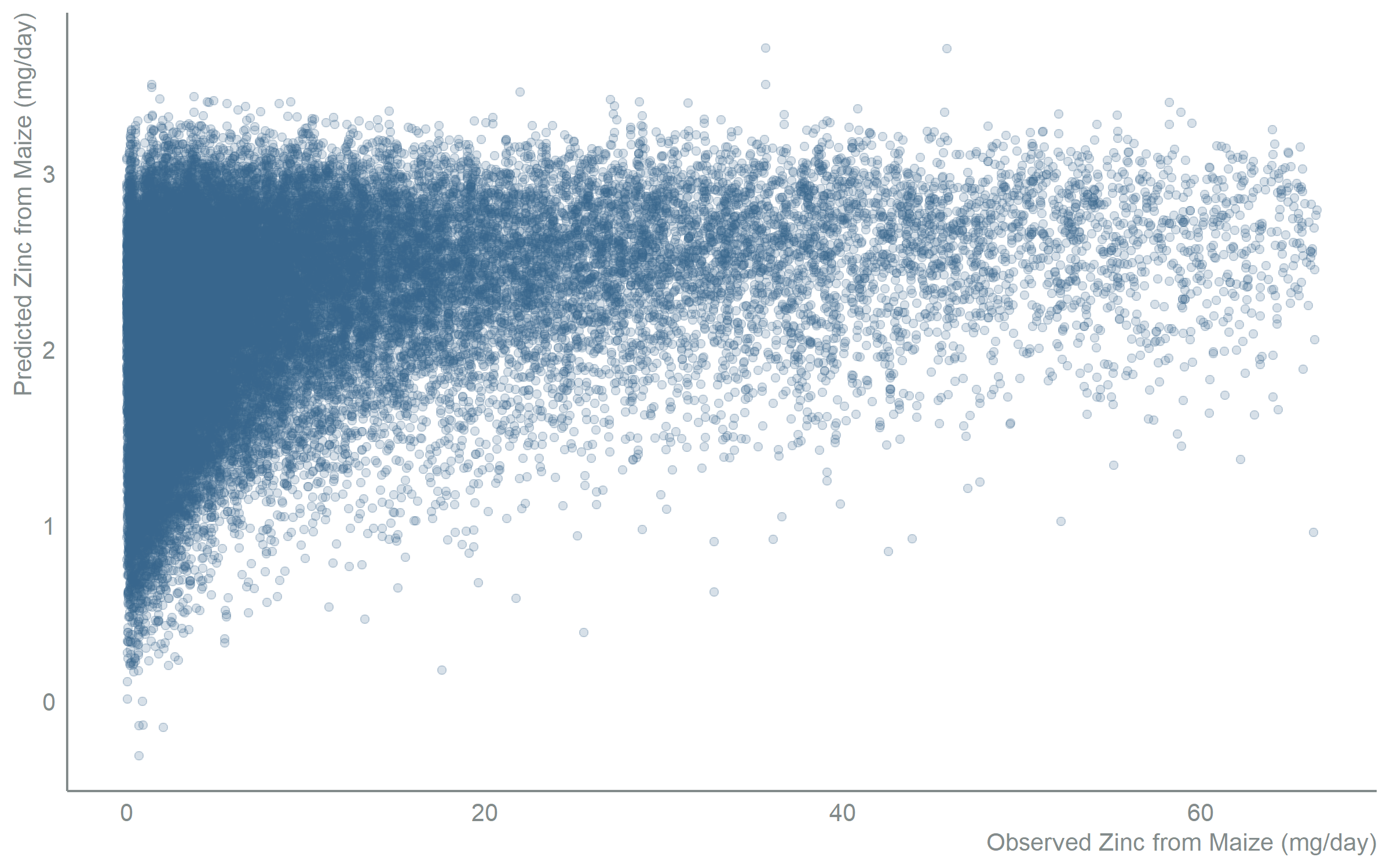
Variable Selection
Not all predictors contribute meaningfully to prediction. We use Wald tests to identify statistically significant variables and remove those that add complexity without improving predictions.
| Variable Significance Testing | |||
| Wald F-test results for zinc intake from maize model | |||
| variable | f_statistic | p_value | significant |
|---|---|---|---|
| parentesco | 10.61 | <0.0001 | * |
| sexo | 44.55 | <0.0001 | * |
| poly(edad, 2) | 147.12 | <0.0001 | * |
| departamento | 6.51 | <0.0001 | * |
| area | 14.93 | 0.0001 | * |
| poly(miembros_hogar, 3) | 0.05 | 0.9840 | |
| propiedad | 1.11 | 0.3504 | |
| poly(grado_estudios_hogar, 3) | 5.83 | 0.0006 | * |
| tipo_vivienda | 8.51 | <0.0001 | * |
| material_paredes | 3.93 | 0.0001 | * |
| material_techo | 6.33 | <0.0001 | * |
| material_piso | 0.25 | 0.9407 | |
| poly(n_cuartos, 3) | 2.00 | 0.1127 | |
| tipo_sanitario | 2.42 | 0.1200 | |
| fuente_agua | 1.45 | 0.1826 | |
| recoleccion_basura | 15.37 | <0.0001 | * |
| electricidad | 0.02 | 0.8903 | |
| televisor | 0.12 | 0.7326 | |
| telefonia_celular | 0.44 | 0.5052 | |
| computadora | 17.94 | <0.0001 | * |
ImportantVariables Retained
11 predictors show significant relationships with zinc intake from maize, spanning demographic, geographic, socioeconomic, housing and asset categories. Variables that do not significantly predict zinc intake from maize after controlling for other factors are excluded from the refined model.
Refined Model
The final model is fitted on the significant predictors alone.
| Zinc Intake from Maize (Refined Model) - Model Coefficients | ||||
| Survey-weighted gamma regression with log link | ||||
| Term | Estimate | Std. Error | t-statistic | p-value |
|---|---|---|---|---|
| (Intercept) | 1.0315 | 0.1938 | 5.3229 | <0.0001 |
| parentescoEsposo(a) o compañero(a) | 0.1760 | 0.0860 | 2.0471 | 0.0408 |
| parentescoHermano(a) | 0.2987 | 0.1538 | 1.9425 | 0.0523 |
| parentescoHijo(a) | 0.3881 | 0.0786 | 4.9400 | <0.0001 |
| parentescoJefe del hogar | 0.1892 | 0.0844 | 2.2428 | 0.0251 |
| parentescoNieto(a) | 0.2641 | 0.0900 | 2.9344 | 0.0034 |
| parentescoOtro no pariente | 0.4555 | 0.4110 | 1.1084 | 0.2679 |
| parentescoOtro pariente | 0.3021 | 0.1244 | 2.4291 | 0.0153 |
| parentescoPadre o madre | 0.3227 | 0.0902 | 3.5768 | 0.0004 |
| parentescoSuegro(a) | 0.3645 | 0.1416 | 2.5746 | 0.0101 |
| parentescoYerno o nuera | 0.3313 | 0.1504 | 2.2028 | 0.0278 |
| sexoMujer | −0.1290 | 0.0203 | −6.3615 | <0.0001 |
| poly(edad, 2)1 | 39.1664 | 4.5423 | 8.6225 | <0.0001 |
| poly(edad, 2)2 | −31.2131 | 2.2632 | −13.7914 | <0.0001 |
| departamentoEl Progreso | 0.2901 | 0.1245 | 2.3312 | 0.0199 |
| departamentoSacatepéquez | 0.3065 | 0.1048 | 2.9253 | 0.0035 |
| departamentoChimaltenango | 0.5173 | 0.1019 | 5.0744 | <0.0001 |
| departamentoEscuintla | 0.2041 | 0.1065 | 1.9167 | 0.0555 |
| departamentoSanta Rosa | 0.4708 | 0.1262 | 3.7294 | 0.0002 |
| departamentoSololá | 0.6202 | 0.1193 | 5.2003 | <0.0001 |
| departamentoTotonicapán | 0.7454 | 0.1116 | 6.6813 | <0.0001 |
| departamentoQuetzaltenango | 0.7724 | 0.1136 | 6.7986 | <0.0001 |
| departamentoSuchitepéquez | 0.5063 | 0.0969 | 5.2258 | <0.0001 |
| departamentoRetalhuleu | 0.6317 | 0.1153 | 5.4790 | <0.0001 |
| departamentoSan Marcos | 0.7276 | 0.1162 | 6.2608 | <0.0001 |
| departamentoHuehuetenango | 0.7412 | 0.1107 | 6.6947 | <0.0001 |
| departamentoQuiché | 0.8287 | 0.1061 | 7.8091 | <0.0001 |
| departamentoBaja Verapaz | 0.7910 | 0.1094 | 7.2282 | <0.0001 |
| departamentoAlta Verapaz | 0.5370 | 0.1165 | 4.6091 | <0.0001 |
| departamentoPetén | 0.7115 | 0.1046 | 6.8020 | <0.0001 |
| departamentoIzabal | 0.5404 | 0.1178 | 4.5888 | <0.0001 |
| departamentoZacapa | 0.1618 | 0.1223 | 1.3235 | 0.1859 |
| departamentoChiquimula | 0.5439 | 0.1293 | 4.2077 | <0.0001 |
| departamentoJalapa | 0.7498 | 0.1215 | 6.1704 | <0.0001 |
| departamentoJutiapa | 0.3934 | 0.1083 | 3.6313 | 0.0003 |
| areaRural | 0.1621 | 0.0401 | 4.0416 | <0.0001 |
| poly(grado_estudios_hogar, 3)1 | −20.5664 | 4.9992 | −4.1139 | <0.0001 |
| poly(grado_estudios_hogar, 3)2 | −1.1251 | 4.4418 | −0.2533 | 0.8001 |
| poly(grado_estudios_hogar, 3)3 | −3.6045 | 4.5038 | −0.8003 | 0.4237 |
| tipo_viviendaApartamento | −0.3108 | 0.1864 | −1.6671 | 0.0957 |
| tipo_viviendaCuarto en casa de vecindad | 0.4160 | 0.3322 | 1.2522 | 0.2107 |
| tipo_viviendaRancho | −1.4949 | 0.2615 | −5.7165 | <0.0001 |
| tipo_viviendaCasa improvisada | 0.2287 | 0.2961 | 0.7724 | 0.4400 |
| material_paredesBlock | 0.2278 | 0.1533 | 1.4862 | 0.1374 |
| material_paredesConcreto | 0.2191 | 0.2731 | 0.8023 | 0.4225 |
| material_paredesAdobe | 0.3880 | 0.1582 | 2.4531 | 0.0143 |
| material_paredesMadera | 0.2694 | 0.1631 | 1.6512 | 0.0989 |
| material_paredesLamina metalica | 0.0231 | 0.3431 | 0.0674 | 0.9463 |
| material_paredesBajareque | 0.6522 | 0.1807 | 3.6098 | 0.0003 |
| material_paredesLepa, palo o caña | 0.5414 | 0.2994 | 1.8081 | 0.0708 |
| material_paredesOtro | −0.0545 | 0.3918 | −0.1390 | 0.8894 |
| material_techoLamina metalica | 0.0149 | 0.0700 | 0.2120 | 0.8321 |
| material_techoAsbesto cemento | −0.0428 | 0.3192 | −0.1342 | 0.8933 |
| material_techoTeja | 0.0378 | 0.0964 | 0.3924 | 0.6948 |
| material_techoPaja, palma o similar | 1.4588 | 0.2657 | 5.4910 | <0.0001 |
| material_techoOtro | −0.2718 | 0.4649 | −0.5848 | 0.5588 |
| recoleccion_basuraLa tiran en cualquier lugar | −0.1694 | 0.0666 | −2.5423 | 0.0111 |
| recoleccion_basuraServicio municipal | −0.3575 | 0.0594 | −6.0226 | <0.0001 |
| recoleccion_basuraServicio privado | −0.4482 | 0.0807 | −5.5506 | <0.0001 |
| computadoraNo | 0.2299 | 0.0536 | 4.2909 | <0.0001 |
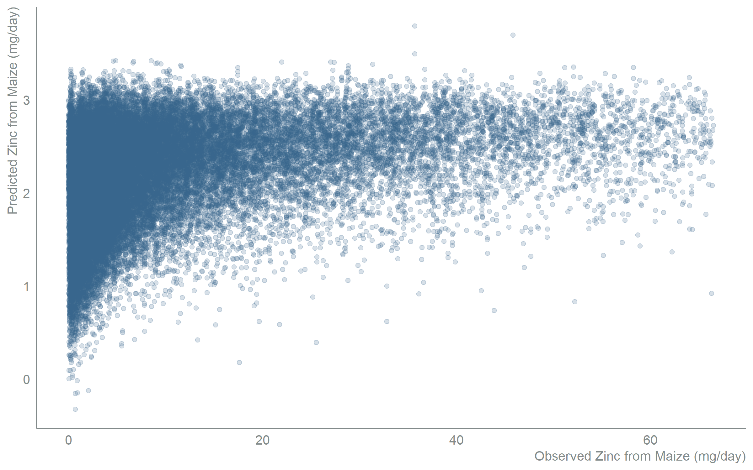
Model Diagnostics
We verify the model meets statistical assumptions:
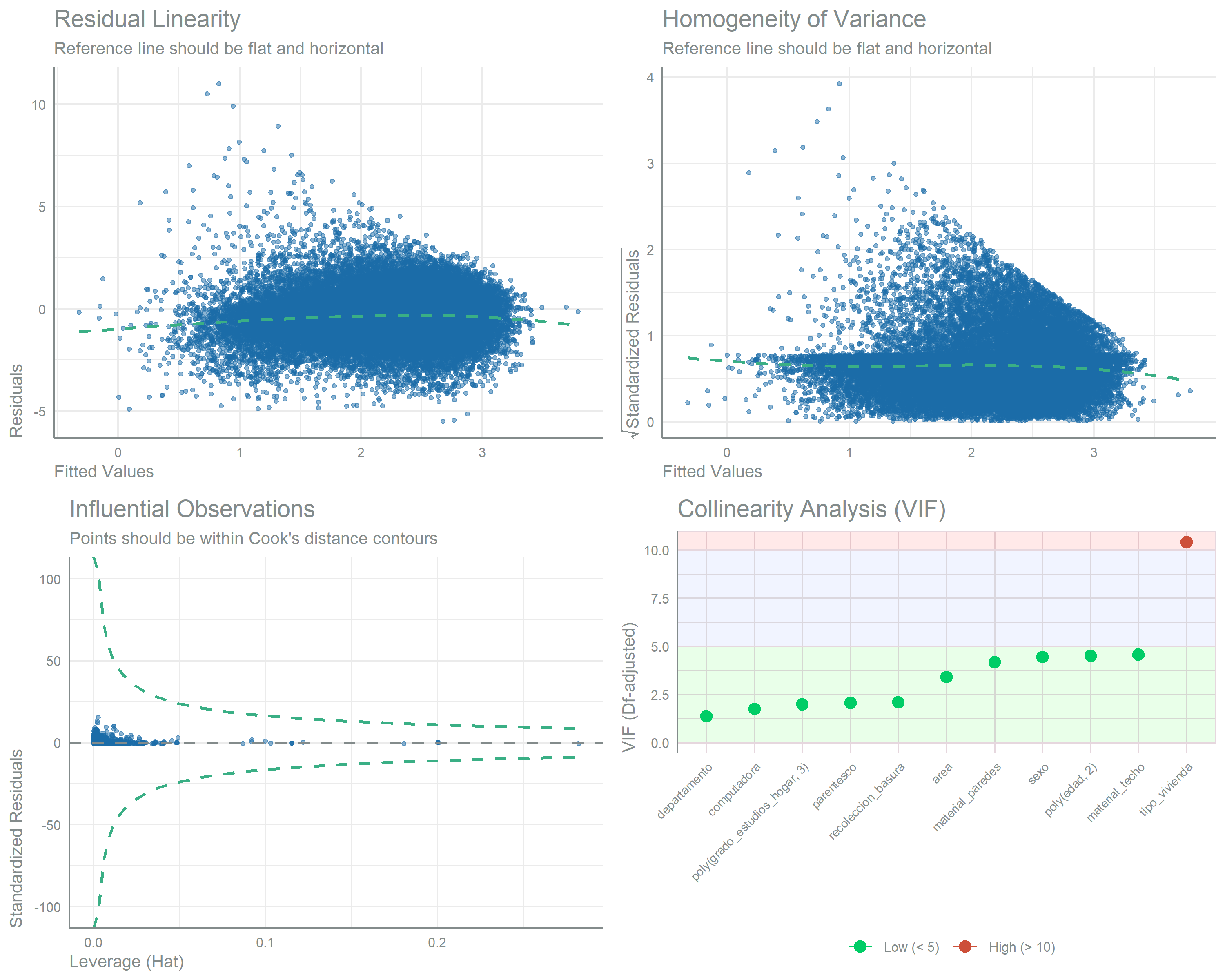
TipDiagnostic Assessment
- Residuals: No systematic patterns, approximately normal
- Leverage: No overly influential observations
- Collinearity: Degrees-of-freedom adjusted variance inflation factors (VIF) reach a maximum of 10.4, with 1 of 11 terms above the conventional threshold of 5
Factors and polynomial terms contribute several columns to the model matrix, so their generalized VIF is rescaled by the term’s degrees of freedom. This places every term on the single-coefficient scale that the thresholds of 5 and 10 refer to.
Modeling Zinc Intake from Non-Maize Sources
Zinc from non-maize sources includes vegetables, fruits, legumes, and animal products. This component remains constant in biofortification scenarios, representing the baseline dietary zinc that would not change with maize interventions.
Distribution Selection
| Distribution Fit Comparison | ||||||
| Goodness-of-fit statistics for Gamma, Lognormal, and Exponential distributions | ||||||
| Distribution | Log-Likelihood |
Information Criteria
|
Goodness-of-Fit Statistics
|
|||
|---|---|---|---|---|---|---|
| AIC | BIC | Kolmogorov-Smirnov | Cramer-von Mises | Anderson-Darling | ||
| Gamma | −96,024.5252 | 192,053.0504 | 192,070.2267 | 0.0175 | 3.2288 | 22.7604 |
| Lognormal | −100,135.1735 | 200,274.3470 | 200,291.5232 | 0.0748 | 82.7171 | 519.8734 |
| Exponential | −97,613.1779 | 195,228.3558 | 195,236.9439 | 0.0975 | 128.9280 | 733.7516 |
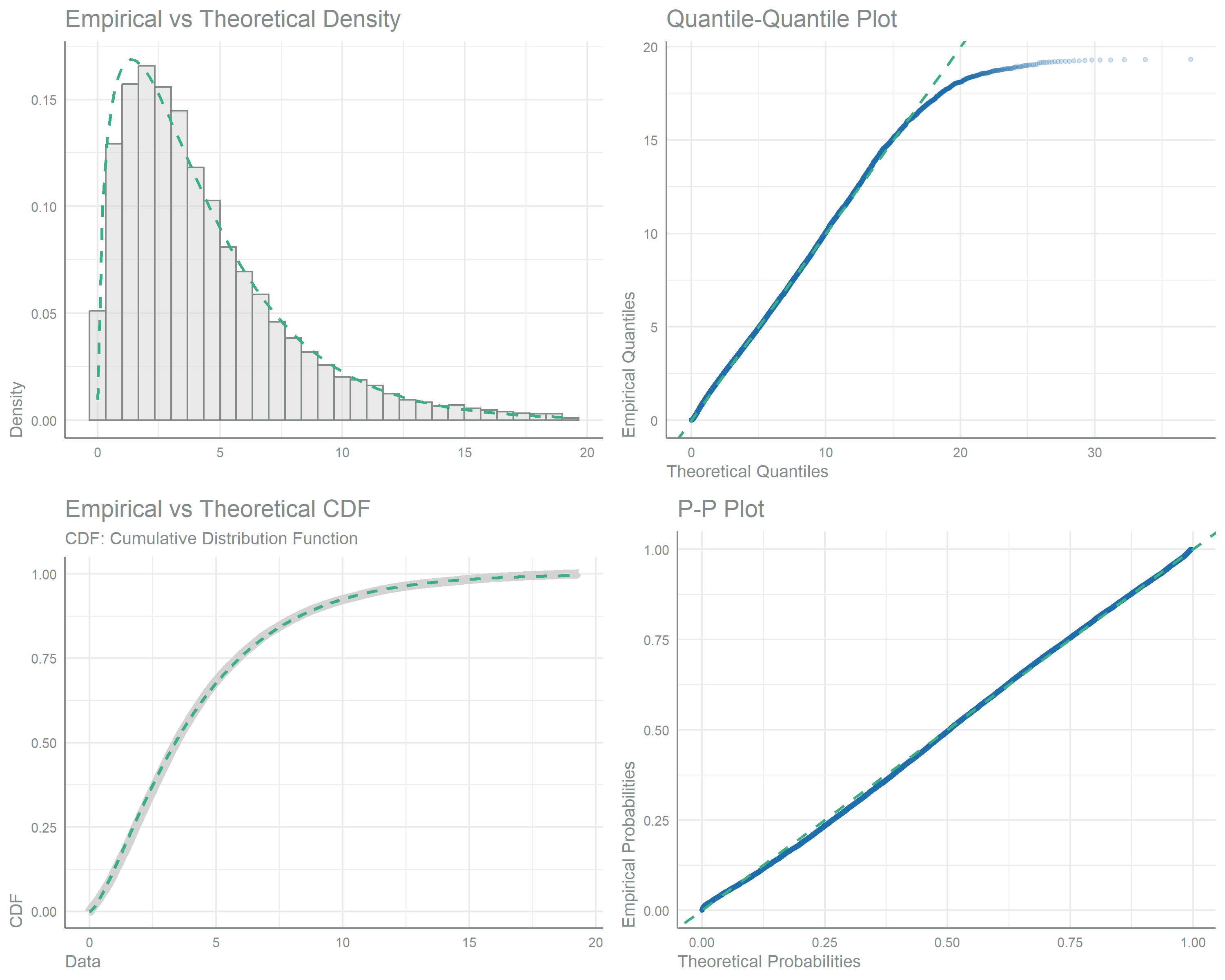
ImportantDistribution Selection
Gamma distribution again provides the best fit for non-maize zinc intake.
Full Model
| Zinc Intake from Non-Maize Sources (Full Model) - Model Coefficients | ||||
| Survey-weighted gamma regression with log link | ||||
| Term | Estimate | Std. Error | t-statistic | p-value |
|---|---|---|---|---|
| (Intercept) | 1.4644 | 0.1146 | 12.7748 | <0.0001 |
| parentescoEsposo(a) o compañero(a) | −0.1800 | 0.0651 | −2.7652 | 0.0058 |
| parentescoHermano(a) | 0.0532 | 0.1109 | 0.4794 | 0.6317 |
| parentescoHijo(a) | −0.0665 | 0.0622 | −1.0694 | 0.2851 |
| parentescoJefe del hogar | −0.1094 | 0.0642 | −1.7031 | 0.0888 |
| parentescoNieto(a) | −0.0844 | 0.0708 | −1.1922 | 0.2334 |
| parentescoOtro no pariente | −0.0663 | 0.2444 | −0.2713 | 0.7862 |
| parentescoOtro pariente | −0.1095 | 0.0743 | −1.4750 | 0.1404 |
| parentescoPadre o madre | −0.1175 | 0.0698 | −1.6838 | 0.0924 |
| parentescoSuegro(a) | 0.0008 | 0.0807 | 0.0102 | 0.9919 |
| parentescoYerno o nuera | 0.1381 | 0.0881 | 1.5687 | 0.1170 |
| sexoMujer | −0.1309 | 0.0103 | −12.7112 | <0.0001 |
| poly(edad, 2)1 | 26.7136 | 2.8550 | 9.3569 | <0.0001 |
| poly(edad, 2)2 | −32.8566 | 1.2718 | −25.8342 | <0.0001 |
| departamentoEl Progreso | 0.0647 | 0.0543 | 1.1917 | 0.2336 |
| departamentoSacatepéquez | 0.1173 | 0.0466 | 2.5163 | 0.0120 |
| departamentoChimaltenango | −0.0323 | 0.0558 | −0.5789 | 0.5627 |
| departamentoEscuintla | 0.1001 | 0.0578 | 1.7316 | 0.0836 |
| departamentoSanta Rosa | 0.1473 | 0.0583 | 2.5271 | 0.0116 |
| departamentoSololá | 0.0267 | 0.0704 | 0.3792 | 0.7046 |
| departamentoTotonicapán | 0.0603 | 0.0655 | 0.9204 | 0.3575 |
| departamentoQuetzaltenango | 0.0283 | 0.0551 | 0.5126 | 0.6083 |
| departamentoSuchitepéquez | −0.0946 | 0.0526 | −1.7993 | 0.0722 |
| departamentoRetalhuleu | 0.0644 | 0.0625 | 1.0312 | 0.3026 |
| departamentoSan Marcos | 0.1274 | 0.0703 | 1.8134 | 0.0700 |
| departamentoHuehuetenango | 0.1711 | 0.0589 | 2.9063 | 0.0037 |
| departamentoQuiché | −0.0328 | 0.0593 | −0.5538 | 0.5798 |
| departamentoBaja Verapaz | −0.0227 | 0.0594 | −0.3823 | 0.7023 |
| departamentoAlta Verapaz | −0.1484 | 0.0685 | −2.1655 | 0.0305 |
| departamentoPetén | −0.0993 | 0.0622 | −1.5962 | 0.1107 |
| departamentoIzabal | 0.0206 | 0.0646 | 0.3189 | 0.7499 |
| departamentoZacapa | −0.0337 | 0.0667 | −0.5048 | 0.6138 |
| departamentoChiquimula | −0.0892 | 0.0719 | −1.2413 | 0.2147 |
| departamentoJalapa | 0.0129 | 0.0574 | 0.2245 | 0.8224 |
| departamentoJutiapa | 0.1230 | 0.0617 | 1.9933 | 0.0464 |
| areaRural | −0.0307 | 0.0253 | −1.2135 | 0.2251 |
| poly(miembros_hogar, 3)1 | −36.4278 | 2.9892 | −12.1863 | <0.0001 |
| poly(miembros_hogar, 3)2 | 2.4626 | 3.9804 | 0.6187 | 0.5362 |
| poly(miembros_hogar, 3)3 | 6.1052 | 4.5193 | 1.3509 | 0.1770 |
| propiedadPropia y pagandola a plazos | −0.0008 | 0.0520 | −0.0148 | 0.9882 |
| propiedadAlquilada | 0.0249 | 0.0332 | 0.7497 | 0.4536 |
| propiedadCedida o prestada | 0.0370 | 0.0326 | 1.1329 | 0.2575 |
| propiedadOtro | −0.1375 | 0.1640 | −0.8384 | 0.4019 |
| poly(grado_estudios_hogar, 3)1 | 4.4967 | 1.9216 | 2.3401 | 0.0194 |
| poly(grado_estudios_hogar, 3)2 | −3.0510 | 1.4990 | −2.0354 | 0.0420 |
| poly(grado_estudios_hogar, 3)3 | −0.1705 | 1.5241 | −0.1119 | 0.9109 |
| tipo_viviendaApartamento | −0.0172 | 0.1655 | −0.1041 | 0.9171 |
| tipo_viviendaCuarto en casa de vecindad | −0.1928 | 0.1080 | −1.7843 | 0.0746 |
| tipo_viviendaRancho | 0.5913 | 0.2133 | 2.7727 | 0.0056 |
| tipo_viviendaCasa improvisada | −0.0219 | 0.2072 | −0.1056 | 0.9159 |
| material_paredesBlock | 0.1869 | 0.0792 | 2.3600 | 0.0184 |
| material_paredesConcreto | 0.2354 | 0.0981 | 2.4006 | 0.0165 |
| material_paredesAdobe | 0.1080 | 0.0849 | 1.2715 | 0.2038 |
| material_paredesMadera | 0.1022 | 0.0885 | 1.1541 | 0.2487 |
| material_paredesLamina metalica | 0.2308 | 0.2256 | 1.0229 | 0.3065 |
| material_paredesBajareque | −0.0941 | 0.1122 | −0.8390 | 0.4016 |
| material_paredesLepa, palo o caña | −0.0595 | 0.2064 | −0.2882 | 0.7732 |
| material_paredesOtro | 0.0752 | 0.1407 | 0.5343 | 0.5933 |
| material_techoLamina metalica | 0.0622 | 0.0311 | 2.0025 | 0.0454 |
| material_techoAsbesto cemento | −0.0656 | 0.1205 | −0.5447 | 0.5861 |
| material_techoTeja | 0.0449 | 0.0578 | 0.7782 | 0.4366 |
| material_techoPaja, palma o similar | −0.4929 | 0.1924 | −2.5623 | 0.0105 |
| material_techoOtro | −0.0302 | 0.2048 | −0.1473 | 0.8829 |
| material_pisoLadrillo de cemento | 0.0504 | 0.0413 | 1.2195 | 0.2229 |
| material_pisoLadrillo de barro | 0.0046 | 0.1107 | 0.0415 | 0.9669 |
| material_pisoTorta de cemento | −0.0120 | 0.0290 | −0.4149 | 0.6783 |
| material_pisoMadera | 0.1562 | 0.1691 | 0.9236 | 0.3559 |
| material_pisoTierra | −0.0622 | 0.0411 | −1.5130 | 0.1305 |
| poly(n_cuartos, 3)1 | 4.8150 | 3.0137 | 1.5977 | 0.1103 |
| poly(n_cuartos, 3)2 | −0.6595 | 2.1485 | −0.3070 | 0.7589 |
| poly(n_cuartos, 3)3 | −0.7773 | 2.2032 | −0.3528 | 0.7243 |
| tipo_sanitarioUso compartido | −0.0327 | 0.0370 | −0.8828 | 0.3775 |
| fuente_aguaTubería fuera de la vivienda | 0.0011 | 0.0372 | 0.0289 | 0.9769 |
| fuente_aguaChorro publico | −0.0088 | 0.0773 | −0.1138 | 0.9094 |
| fuente_aguaPozo perforado | 0.0427 | 0.0405 | 1.0536 | 0.2923 |
| fuente_aguaRío, lago, manantial | −0.1905 | 0.0721 | −2.6433 | 0.0083 |
| fuente_aguaCamion cisterna | 0.0702 | 0.0643 | 1.0922 | 0.2749 |
| fuente_aguaAgua de lluvia | −0.0211 | 0.0791 | −0.2669 | 0.7896 |
| fuente_aguaOtro | −0.1156 | 0.0550 | −2.1017 | 0.0358 |
| recoleccion_basuraLa tiran en cualquier lugar | −0.0208 | 0.0574 | −0.3614 | 0.7179 |
| recoleccion_basuraServicio municipal | 0.0036 | 0.0273 | 0.1308 | 0.8960 |
| recoleccion_basuraServicio privado | 0.0423 | 0.0345 | 1.2242 | 0.2211 |
| electricidadNo | −0.0269 | 0.0381 | −0.7068 | 0.4798 |
| televisorNo | −0.0648 | 0.0212 | −3.0546 | 0.0023 |
| telefonia_celularNo | −0.0389 | 0.0242 | −1.6061 | 0.1085 |
| computadoraNo | −0.0605 | 0.0283 | −2.1393 | 0.0326 |
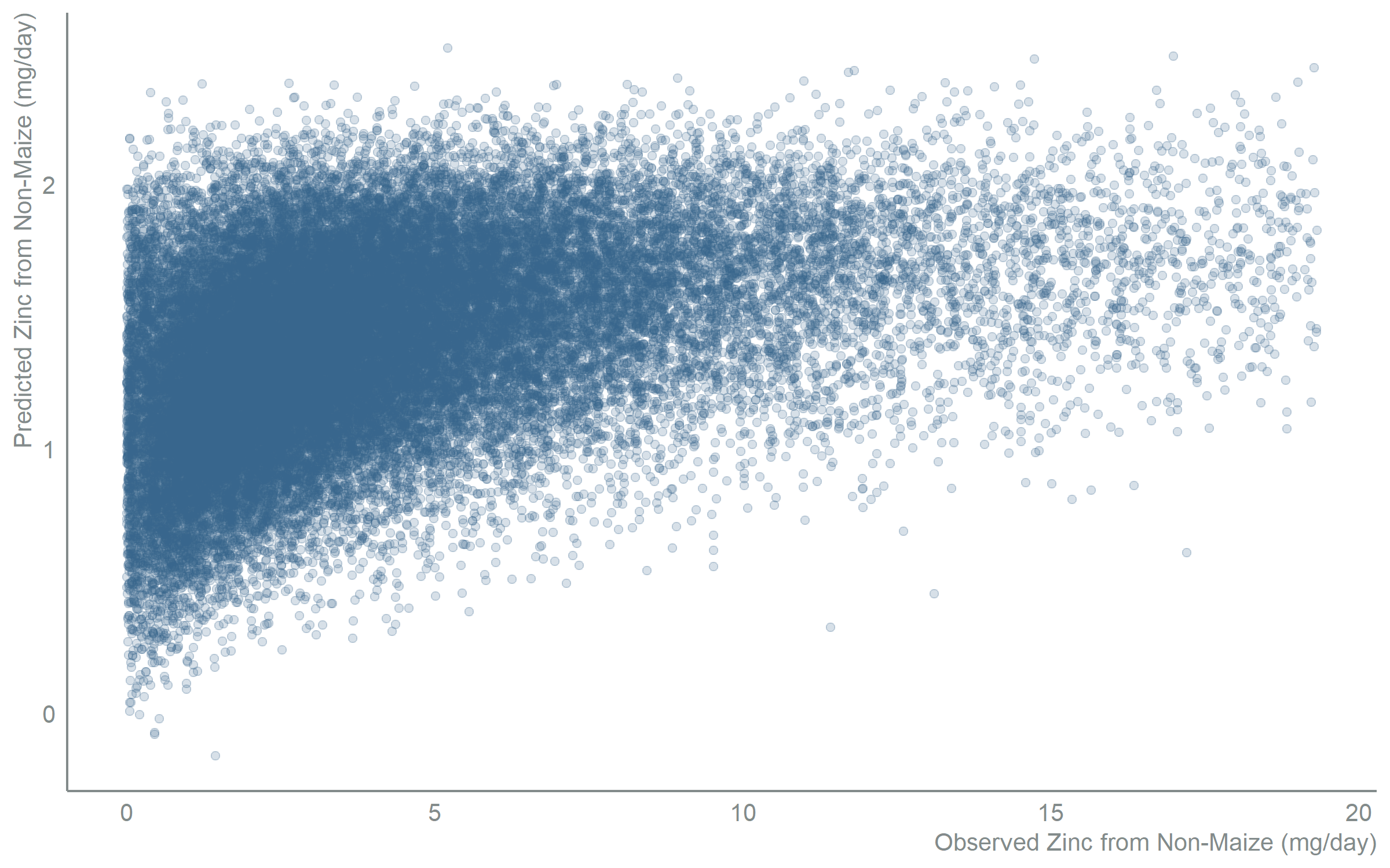
Variable Selection
| Variable Significance Testing | |||
| Wald F-test results for zinc intake from non-maize model | |||
| variable | f_statistic | p_value | significant |
|---|---|---|---|
| parentesco | 10.53 | <0.0001 | * |
| sexo | 161.57 | <0.0001 | * |
| poly(edad, 2) | 347.33 | <0.0001 | * |
| departamento | 3.61 | <0.0001 | * |
| area | 1.47 | 0.2251 | |
| poly(miembros_hogar, 3) | 120.74 | <0.0001 | * |
| propiedad | 0.62 | 0.6502 | |
| poly(grado_estudios_hogar, 3) | 2.61 | 0.0503 | |
| tipo_vivienda | 5.33 | 0.0003 | * |
| material_paredes | 3.30 | 0.0010 | * |
| material_techo | 2.65 | 0.0215 | * |
| material_piso | 1.40 | 0.2218 | |
| poly(n_cuartos, 3) | 1.22 | 0.3023 | |
| tipo_sanitario | 0.78 | 0.3775 | |
| fuente_agua | 1.91 | 0.0645 | |
| recoleccion_basura | 0.66 | 0.5750 | |
| electricidad | 0.50 | 0.4798 | |
| televisor | 9.33 | 0.0023 | * |
| telefonia_celular | 2.58 | 0.1085 | |
| computadora | 4.58 | 0.0326 | * |
ImportantVariables Retained
10 predictors significantly predict zinc intake from non-maize sources, drawing from the same set of demographic, geographic, socioeconomic and housing variables. The retained set differs from the maize model: the two outcomes are predicted by different subsets of the same candidate variables.
Refined Model
| Zinc Intake from Non-Maize Sources (Refined Model) - Model Coefficients | ||||
| Survey-weighted gamma regression with log link | ||||
| Term | Estimate | Std. Error | t-statistic | p-value |
|---|---|---|---|---|
| (Intercept) | 1.6273 | 0.1108 | 14.6935 | <0.0001 |
| parentescoEsposo(a) o compañero(a) | −0.2050 | 0.0671 | −3.0554 | 0.0023 |
| parentescoHermano(a) | 0.0381 | 0.1088 | 0.3506 | 0.7260 |
| parentescoHijo(a) | −0.0868 | 0.0646 | −1.3448 | 0.1789 |
| parentescoJefe del hogar | −0.1362 | 0.0666 | −2.0457 | 0.0410 |
| parentescoNieto(a) | −0.1028 | 0.0732 | −1.4044 | 0.1604 |
| parentescoOtro no pariente | −0.0191 | 0.2550 | −0.0749 | 0.9403 |
| parentescoOtro pariente | −0.1193 | 0.0767 | −1.5541 | 0.1204 |
| parentescoPadre o madre | −0.1329 | 0.0719 | −1.8483 | 0.0648 |
| parentescoSuegro(a) | −0.0143 | 0.0812 | −0.1766 | 0.8599 |
| parentescoYerno o nuera | 0.1013 | 0.0908 | 1.1147 | 0.2652 |
| sexoMujer | −0.1333 | 0.0106 | −12.5344 | <0.0001 |
| poly(edad, 2)1 | 27.5131 | 2.7332 | 10.0663 | <0.0001 |
| poly(edad, 2)2 | −33.3262 | 1.2846 | −25.9425 | <0.0001 |
| departamentoEl Progreso | 0.0261 | 0.0511 | 0.5111 | 0.6094 |
| departamentoSacatepéquez | 0.1034 | 0.0459 | 2.2523 | 0.0245 |
| departamentoChimaltenango | −0.0690 | 0.0533 | −1.2950 | 0.1956 |
| departamentoEscuintla | 0.0703 | 0.0518 | 1.3580 | 0.1747 |
| departamentoSanta Rosa | 0.0870 | 0.0539 | 1.6156 | 0.1064 |
| departamentoSololá | −0.0278 | 0.0660 | −0.4207 | 0.6740 |
| departamentoTotonicapán | −0.0026 | 0.0605 | −0.0438 | 0.9651 |
| departamentoQuetzaltenango | −0.0304 | 0.0503 | −0.6041 | 0.5459 |
| departamentoSuchitepéquez | −0.1339 | 0.0468 | −2.8584 | 0.0043 |
| departamentoRetalhuleu | 0.0335 | 0.0567 | 0.5918 | 0.5541 |
| departamentoSan Marcos | 0.0441 | 0.0653 | 0.6746 | 0.5000 |
| departamentoHuehuetenango | 0.0988 | 0.0526 | 1.8801 | 0.0603 |
| departamentoQuiché | −0.0970 | 0.0538 | −1.8011 | 0.0719 |
| departamentoBaja Verapaz | −0.0831 | 0.0581 | −1.4322 | 0.1523 |
| departamentoAlta Verapaz | −0.2443 | 0.0627 | −3.8944 | 0.0001 |
| departamentoPetén | −0.1472 | 0.0602 | −2.4463 | 0.0146 |
| departamentoIzabal | −0.0233 | 0.0627 | −0.3717 | 0.7102 |
| departamentoZacapa | −0.0906 | 0.0656 | −1.3818 | 0.1673 |
| departamentoChiquimula | −0.1577 | 0.0692 | −2.2804 | 0.0227 |
| departamentoJalapa | −0.0617 | 0.0529 | −1.1679 | 0.2431 |
| departamentoJutiapa | 0.0751 | 0.0585 | 1.2829 | 0.1998 |
| poly(miembros_hogar, 3)1 | −37.0274 | 2.6447 | −14.0006 | <0.0001 |
| poly(miembros_hogar, 3)2 | 1.9885 | 3.6923 | 0.5386 | 0.5903 |
| poly(miembros_hogar, 3)3 | 6.3435 | 4.2467 | 1.4937 | 0.1355 |
| tipo_viviendaApartamento | −0.0168 | 0.1692 | −0.0994 | 0.9208 |
| tipo_viviendaCuarto en casa de vecindad | −0.2232 | 0.0998 | −2.2368 | 0.0255 |
| tipo_viviendaRancho | 0.5335 | 0.2142 | 2.4913 | 0.0128 |
| tipo_viviendaCasa improvisada | −0.0526 | 0.2061 | −0.2554 | 0.7985 |
| material_paredesBlock | 0.1514 | 0.0822 | 1.8424 | 0.0656 |
| material_paredesConcreto | 0.2017 | 0.1002 | 2.0117 | 0.0444 |
| material_paredesAdobe | 0.0282 | 0.0871 | 0.3237 | 0.7462 |
| material_paredesMadera | −0.0024 | 0.0893 | −0.0268 | 0.9786 |
| material_paredesLamina metalica | 0.1682 | 0.2263 | 0.7435 | 0.4573 |
| material_paredesBajareque | −0.1926 | 0.1144 | −1.6831 | 0.0926 |
| material_paredesLepa, palo o caña | −0.1858 | 0.2045 | −0.9083 | 0.3639 |
| material_paredesOtro | −0.0197 | 0.1392 | −0.1416 | 0.8874 |
| material_techoLamina metalica | 0.0244 | 0.0271 | 0.8971 | 0.3698 |
| material_techoAsbesto cemento | −0.0519 | 0.1245 | −0.4165 | 0.6771 |
| material_techoTeja | 0.0173 | 0.0546 | 0.3164 | 0.7517 |
| material_techoPaja, palma o similar | −0.5211 | 0.1921 | −2.7125 | 0.0068 |
| material_techoOtro | −0.0952 | 0.2016 | −0.4721 | 0.6369 |
| televisorNo | −0.0865 | 0.0215 | −4.0326 | <0.0001 |
| computadoraNo | −0.0935 | 0.0270 | −3.4556 | 0.0006 |
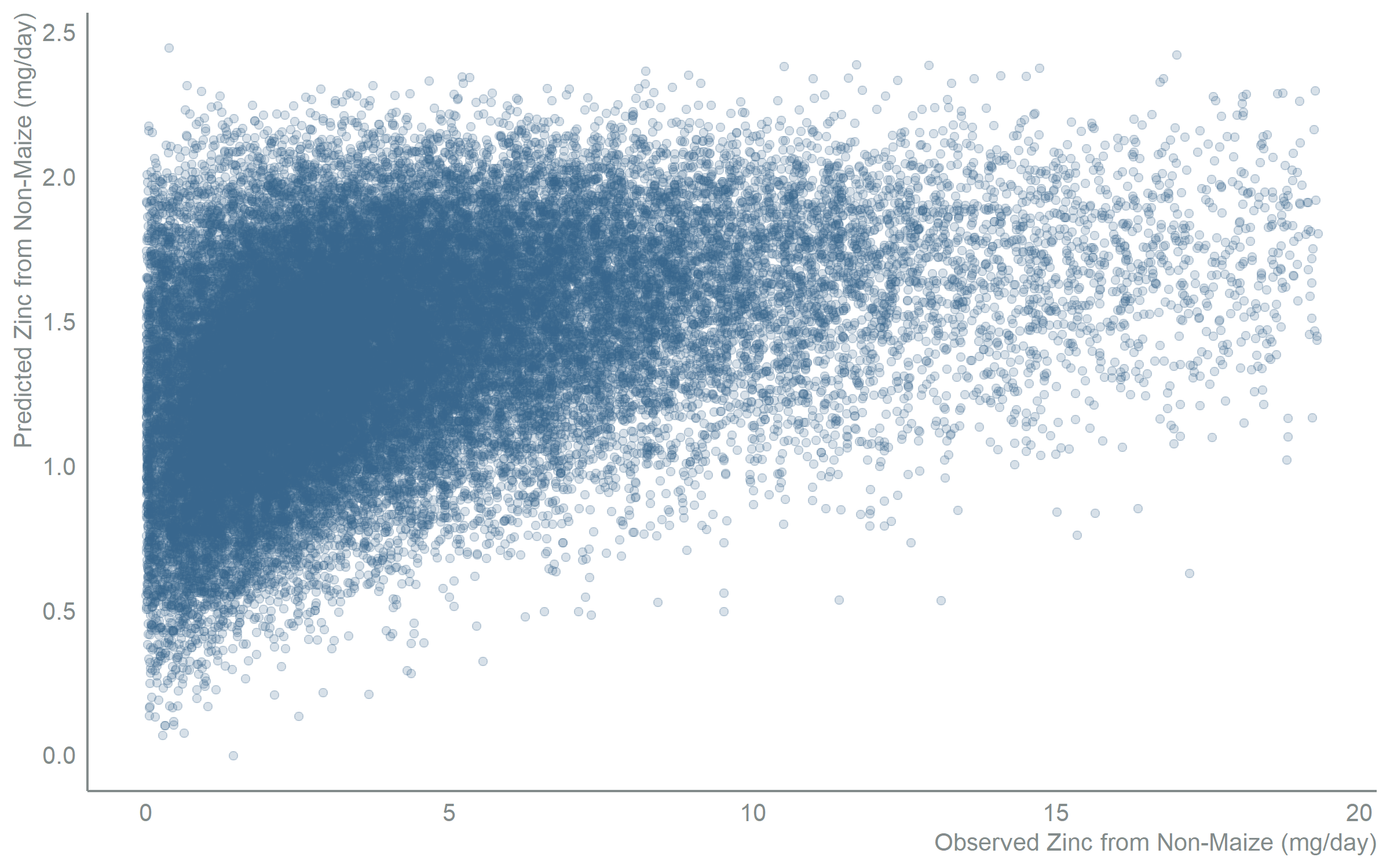
Model Diagnostics
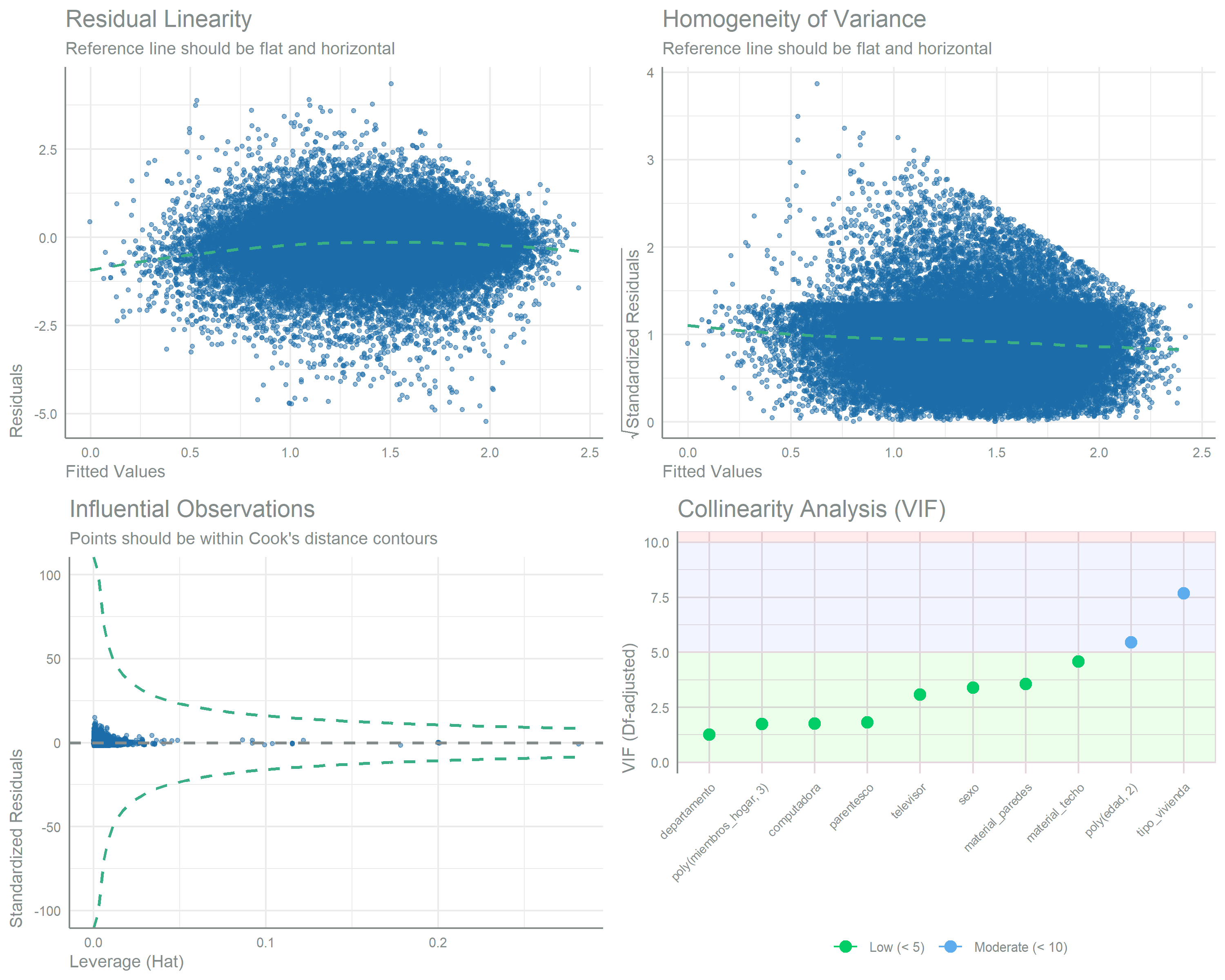
Summary
Final Model Performance
| Final Model Performance | ||
| Refined gamma regression with log link | ||
| Metric | Zinc from maize | Zinc from non-maize |
|---|---|---|
| N observations | 39,661 | 39,661 |
| N predictors | 59 | 56 |
| Pseudo-R² (McFadden)1 | 0.191 | 0.155 |
| Pseudo-R² (Cragg-Uhler)2 | 0.332 | 0.207 |
| AIC | 53,434 | 25,395 |
| Dispersion | 1.653 | 0.548 |
| 1 Pseudo-R² (McFadden) = 1 − (residual deviance / null deviance). Conservative measure; values above 0.2 are conventionally considered good for GLMs. | ||
| 2 Pseudo-R² (Cragg-Uhler), also known as Nagelkerke's R², is normalized to a [0, 1] range and generally yields higher values than McFadden. Both measures are reported for transparency. | ||
Model Comparison
| Outcome | Final Predictors | Retained predictors (examples) |
|---|---|---|
| Zinc from maize | 11 variables | Age, department, education, area, garbage collection |
| Zinc from non-maize | 10 variables | Age, household size, dwelling type, wall materials |
Key Findings
Higher maize share for zinc: The proportion of zinc intake from maize is higher than for iron (see Daily Nutrient Intake by Source in Module 1), which makes a larger fraction of zinc intake biofortification-modifiable
Geographic variation: Department is retained in both models, consistent with regional variation in dietary patterns
Differential role of area: Urban/rural area is retained in the maize model and not in the non-maize model, so it carries predictive power for one intake source and not the other
Service and asset variables: Garbage collection and computer ownership are retained in the maize model, television and computer ownership in the non-maize model
Application
These models will be applied to SIVESNU 2018 children to predict their zinc intake profiles based on their demographic and socioeconomic characteristics. The predicted values enable linking nutritional status to stunting outcomes.