Prepare SIVESNU Height Data

Module 5: Meta-analysis

Why Prepare SIVESNU Height Data?

The Meta-analysis (Gunaratna) pathway requires a model that predicts child height from socioeconomic and demographic variables. This model will be trained on SIVESNU 2018 — which contains direct anthropometric measurements — and applied to children in the ENCOVI 2023 dataset, who lack height data but have comparable socioeconomic profiles.

The predictor variable set comprises demographic, socioeconomic, and geographic indicators present in both surveys, constituting the bridge for cross-dataset prediction. The hypothesis is that the same variables predicting nutrient intakes (transfer models) also predict child stature, since socioeconomic conditions are linked to both dietary quality and growth outcomes.

This document describes the preparation of the SIVESNU training dataset through six stages: population filtering, variable harmonization, missing value imputation, predictor quality assessment, normalization, and feature selection.

Target Population

SIVESNU 2018 includes anthropometric measurements for children under 5 years. We filter to the study population (6-59 months) and require valid height and height-for-age z-score data, resulting in 773 children available for model training.

Children under 6 months are excluded as they should be exclusively breastfed per WHO guidelines, making their anthropometric patterns non-comparable with older children’s dietary intake profiles.

Table 1: Target population summary after filtering

Target Population Filtering Summary. SIVESNU 2018 children aged 6-59 months with valid anthropometry
Metric	N
Target Population Filtering Summary
SIVESNU 2018 children aged 6-59 months with valid anthropometry
Total children in SIVESNU child table	902
Children aged 6-59 months	812
With valid height measurement	773
With valid ZLEN z-score	773
Final target population	773

Population Yield

The filtering pipeline retains 773 of 902 children (85.7%). The age restriction (6-59 months) accounts for most of the attrition, removing 90 children, and a further 39 records lack a height measurement. Every child with a valid height also carries a valid height-for-age z-score, so the two criteria select the same records.

Variable Harmonization

SIVESNU and ENCOVI use different variable naming conventions and coding schemes. We harmonize SIVESNU variables to match the coding structure used in ENCOVI 2023, so that the trained height model applies across surveys without recoding. The harmonization covers geographic classification, household characteristics, housing materials, basic services, and household assets.

Table 2: Merge quality assessment

Child-Household Merge Quality. Matching children to their household socioeconomic profiles
Metric	Value
Child-Household Merge Quality
Matching children to their household socioeconomic profiles
Children before merge	773
Children after merge	773
Match rate	100%
Children with complete department	771
Children with complete area	770

Merge Quality

The 773 children match to their household socioeconomic profiles at a rate of 100%. Department and area classification are close to complete, at 771 and 770 records respectively, leaving 2 and 3 records without a geographic identifier.

Missing Value Treatment

Missing Value Diagnosis

Missing data is minimal across predictor variables. The four variables with any missing values — fuente_agua, area, departamento, and tipo_vivienda — each affect fewer than 1% of records.

Table 3: Missing value summary for predictor variables

Missing Values in Predictor Variables. Assessment prior to imputation
Variable	N Missing	% Missing
Missing Values in Predictor Variables
Assessment prior to imputation
fuente_agua	4	0.52%
area	3	0.39%
departamento	2	0.26%
tipo_vivienda	2	0.26%
parentesco	0	0.00%
sexo	0	0.00%
edad	0	0.00%
miembros_hogar	0	0.00%
grado_estudios_hogar	0	0.00%
propiedad	0	0.00%
material_paredes	0	0.00%
material_techo	0	0.00%
material_piso	0	0.00%
n_cuartos	0	0.00%
cocina	0	0.00%
tipo_sanitario	0	0.00%
recoleccion_basura	0	0.00%
electricidad	0	0.00%
televisor	0	0.00%
telefonia_fija	0	0.00%
telefonia_celular	0	0.00%
computadora	0	0.00%

Random Forest Imputation

Missing values are imputed via Random Forest using the impute_rf_parallel() utility function, which wraps missRanger::missRanger() with a multi-threaded ranger engine. The procedure preserves inter-variable correlations and handles mixed data types, continuous and categorical, simultaneously. Imputation quality is summarized via out-of-bag (OOB) error metrics — OOBE for continuous variables and the proportion of falsely classified entries (PFC) for categorical variables.

Table 4: Random Forest imputation quality metrics

Missing Value Imputation Quality Assessment. Out-of-bag error estimates from Random Forest imputation (missRanger)
Metric	Value	Quality Assessment
Missing Value Imputation Quality Assessment
Out-of-bag error estimates from Random Forest imputation (missRanger)
OOBE (Continuous Variables)¹	N/A	No continuous variables required imputation
PFC (Categorical Variables)²	0.3171	Review required
Number of Iterations	10	Fixed parameter
Trees per Iteration	100	Fixed parameter
¹ OOBE: aggregated out-of-bag error across the continuous variables imputed, bounded in [0, 1] and invariant to their scale. Values < 0.5 indicate acceptable imputation quality for continuous variables. N/A when no continuous variables had missing values.
² PFC: Proportion of Falsely Classified entries. Values < 0.2 indicate acceptable imputation quality for categorical variables.

Reading the Two Metrics

Out-of-bag (OOB) error is computed from observations randomly excluded during tree construction, which gives an internal quality metric without a separate test set.

The continuous metric is reported as N/A: the two continuous predictors (miembros_hogar, n_cuartos) had no missing values, so no continuous imputation was required.

The categorical metric is 0.3171, above the 0.2 reference value, and the table flags it for review. It is the OOB misclassification rate of the forests fitted for the four variables that carry missing values, so it measures how predictable those variables are from the rest of the predictor set, not the accuracy of the specific cells filled. Those cells number 11 across 773 records.

Predictor Quality Assessment

Correlation Structure

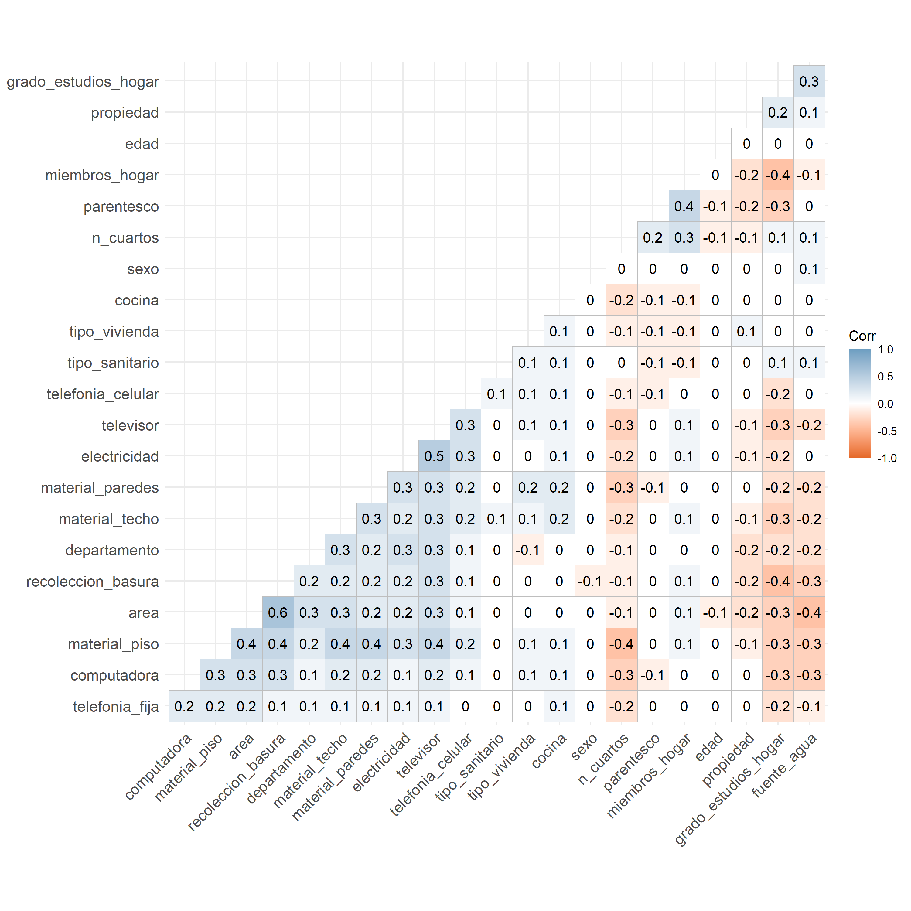
We assess pairwise correlation among predictor variables to identify potential multicollinearity. Pairs correlating above 0.8 are candidates for removal.

Correlation heatmap showing the lower triangle of pairwise correlations among the predictor variables, with variables hierarchically clustered along both axes and each cell labelled with its coefficient. Color runs from orange for negative through white at zero to blue for positive correlations. Most pairs are weak; housing quality indicators (materials, assets, services) form a block of moderate positive correlations while demographic variables stay largely independent. The strongest pair is 0.6, recoleccion_basura with area, below the 0.8 multicollinearity screen. — Figure 1: Correlation matrix of predictor variables for height modeling

Correlation Patterns

The highest pairwise correlation is 0.6 (recoleccion_basura with area), below the 0.8 value above which pairs become candidates for removal. Housing quality indicators cluster together (materials, assets, services), while demographic variables (edad, sexo, parentesco) stay largely independent of the socioeconomic indicators. No variable pair is removed on correlation grounds.

Near-Zero Variance Analysis

Variables with near-zero variance provide minimal discriminating information for the transfer model and can introduce noise in feature selection.

Table 5: Near-zero variance analysis for predictor variables

Near-Zero Variance Analysis. Variables with insufficient variation for modeling
Variable	Frequency Ratio	% Unique Values	Zero Variance	Near-Zero Variance
Near-Zero Variance Analysis
Variables with insufficient variation for modeling
tipo_vivienda	56.62	0.65	FALSE	TRUE
telefonia_fija	29.92	0.26	FALSE	TRUE
computadora	8.66	0.26	FALSE	FALSE
telefonia_celular	7.99	0.26	FALSE	FALSE
electricidad	6.09	0.26	FALSE	FALSE
propiedad	5.37	0.65	FALSE	FALSE
cocina	5.13	0.26	FALSE	FALSE
material_techo	5.13	0.65	FALSE	FALSE
recoleccion_basura	3.91	0.52	FALSE	FALSE
tipo_sanitario	3.89	0.26	FALSE	FALSE
material_paredes	3.47	1.03	FALSE	FALSE
parentesco	2.65	0.78	FALSE	FALSE
grado_estudios_hogar	2.32	1.29	FALSE	FALSE
area	2.28	0.26	FALSE	FALSE
televisor	2.25	0.26	FALSE	FALSE
departamento	1.63	2.85	FALSE	FALSE
n_cuartos	1.56	1.29	FALSE	FALSE
material_piso	1.51	0.78	FALSE	FALSE
fuente_agua	1.30	1.03	FALSE	FALSE
miembros_hogar	1.08	2.20	FALSE	FALSE
sexo	1.05	0.26	FALSE	FALSE
edad	1.00	79.56	FALSE	FALSE
Variables flagged as near-zero variance will be removed from the modeling dataset.

Variables Removed

Two variables are flagged as near-zero variance and removed from the modeling dataset: tipo_vivienda (frequency ratio 56.62 — dominated by “Casa formal”) and telefonia_fija (frequency ratio 29.92 — nearly all households lack landlines). The remaining 20 variables proceed to normalization and feature selection.

Continuous Variable Normalization

The two continuous predictors (miembros_hogar and n_cuartos) are normalized to reduce skewness. bestNormalize() evaluates a family of candidate transformations for each variable and keeps the one that comes closest to normality; the Transformation Type column reports which one it selected. The fitted objects are saved and reapplied to ENCOVI data in the transfer step, so both surveys enter the model on the same scale.

Table 6: Yeo-Johnson transformation summary

Yeo-Johnson Transformation Results. Normalization of continuous predictor variables
Variable	Pre-transform Skewness	Post-transform Skewness	Transformation Type
Yeo-Johnson Transformation Results
Normalization of continuous predictor variables
miembros_hogar	1.278	1.278	center_scale
n_cuartos	1.724	0.097	boxcox

Transformation Outcomes

Skewness in n_cuartos falls from 1.724 to 0.097 under the transformation. For miembros_hogar the procedure selects a centre-scale normalization, which leaves the skewness at its original value of 1.278: household size is a count with a short right tail, and the location-scale shift does not change its shape.

Feature Selection

Boruta Algorithm

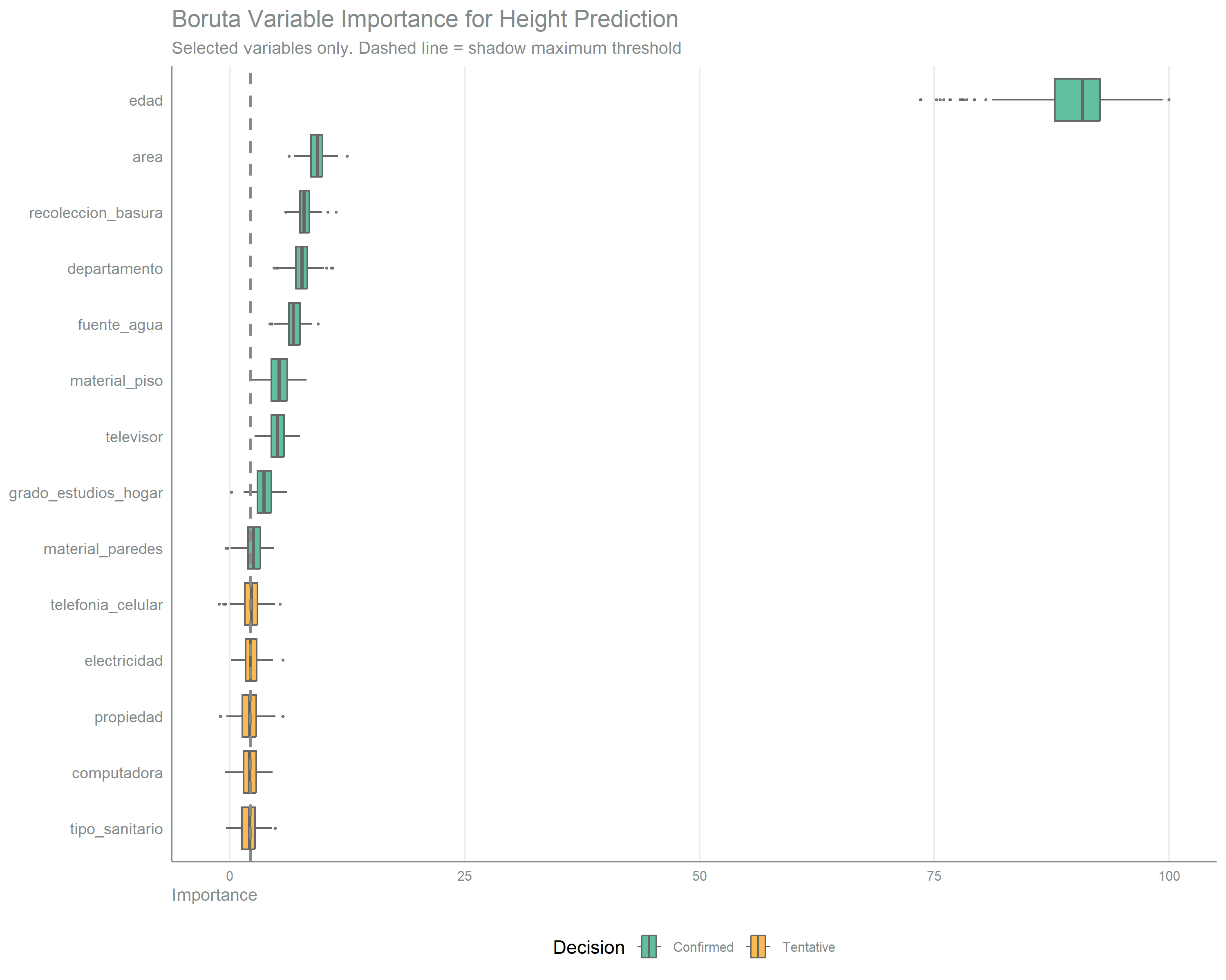
The Boruta algorithm evaluates each candidate predictor against random shadow variables to determine statistical relevance for height prediction. Feature selection uses raw height in centimetres (talla_cm) as the outcome, which is the variable transferred to ENCOVI, and keeps the selection independent of age: height-for-age z-scores are age-standardized, and age is itself a predictor. The implementation uses Boruta::getImpRfZ as the importance source, which delegates the variable importance computation to the multi-threaded ranger backend.

Table 7: Boruta feature selection results for height prediction

Boruta Feature Selection Results. Variable importance assessment for height (talla_cm) prediction
Metric	Value
Boruta Feature Selection Results
Variable importance assessment for height (talla_cm) prediction
Variables evaluated	20
Confirmed (relevant)	9
Tentative (borderline)	5
Rejected (not relevant)	6
Variables selected (Confirmed + Tentative)	14
Method: Boruta with ranger importance source (multi-threaded), 150 iterations against shadow variables

Horizontal boxplot chart ranking the selected predictor variables by Boruta importance, with importance on the x-axis and one box per variable on the y-axis. Boxes are colored by decision: green for confirmed and yellow for tentative. A dashed vertical line marks the shadow-maximum threshold that variables must exceed to be retained. Age (edad) dominates with importance an order of magnitude above all others, followed by a secondary cluster of geographic and housing quality indicators. — Figure 2: Variable importance from Boruta feature selection for height prediction

Feature Selection Results

Of 20 candidate predictors, Boruta confirms 9 as relevant and classifies 5 as tentative (borderline), yielding 14 selected variables. Age (edad) reaches a median importance of 90.8, an order of magnitude above the next variable, which is consistent with the developmental relationship between age and height. Geographic (area, departamento) and housing quality indicators (recoleccion_basura, fuente_agua, material_piso) form a secondary cluster in the 5 to 9 range, carrying the socioeconomic gradient associated with growth beyond what age accounts for.

Final Modeling Dataset

The selected predictors, outcome variable, and validation references are consolidated into a single modeling-ready dataset. Three protected variables — edad, departamento, and sexo — are retained regardless of their Boruta decision because transferring height to ENCOVI requires them: edad and sexo for the WHO LMS lookup, and departamento for survey weight recalibration.

Table 8: Final modeling dataset summary

Final Modeling Dataset Structure. Variables retained in the SIVESNU height modeling dataset
Category	Variables	N
Final Modeling Dataset Structure
Variables retained in the SIVESNU height modeling dataset
Identifiers & metadata	nboletahogar, conglomerado, pesonino, edad_mes	4
Outcome variable	talla_cm	1
Validation references (not predictors)	zlen, hfa	2
Selected predictors	edad, area, recoleccion_basura, departamento, fuente_agua, material_piso, televisor, grado_estudios_hogar, material_paredes, telefonia_celular, electricidad, propiedad, computadora, tipo_sanitario, sexo	15
Original continuous values (reference)	miembros_hogar_original, n_cuartos_original	2
TOTAL		24

Height Distribution by Stunting Status

The final visualization shows how height is distributed by stunting status within each age group, which is the variation the transfer model is asked to reproduce in ENCOVI.

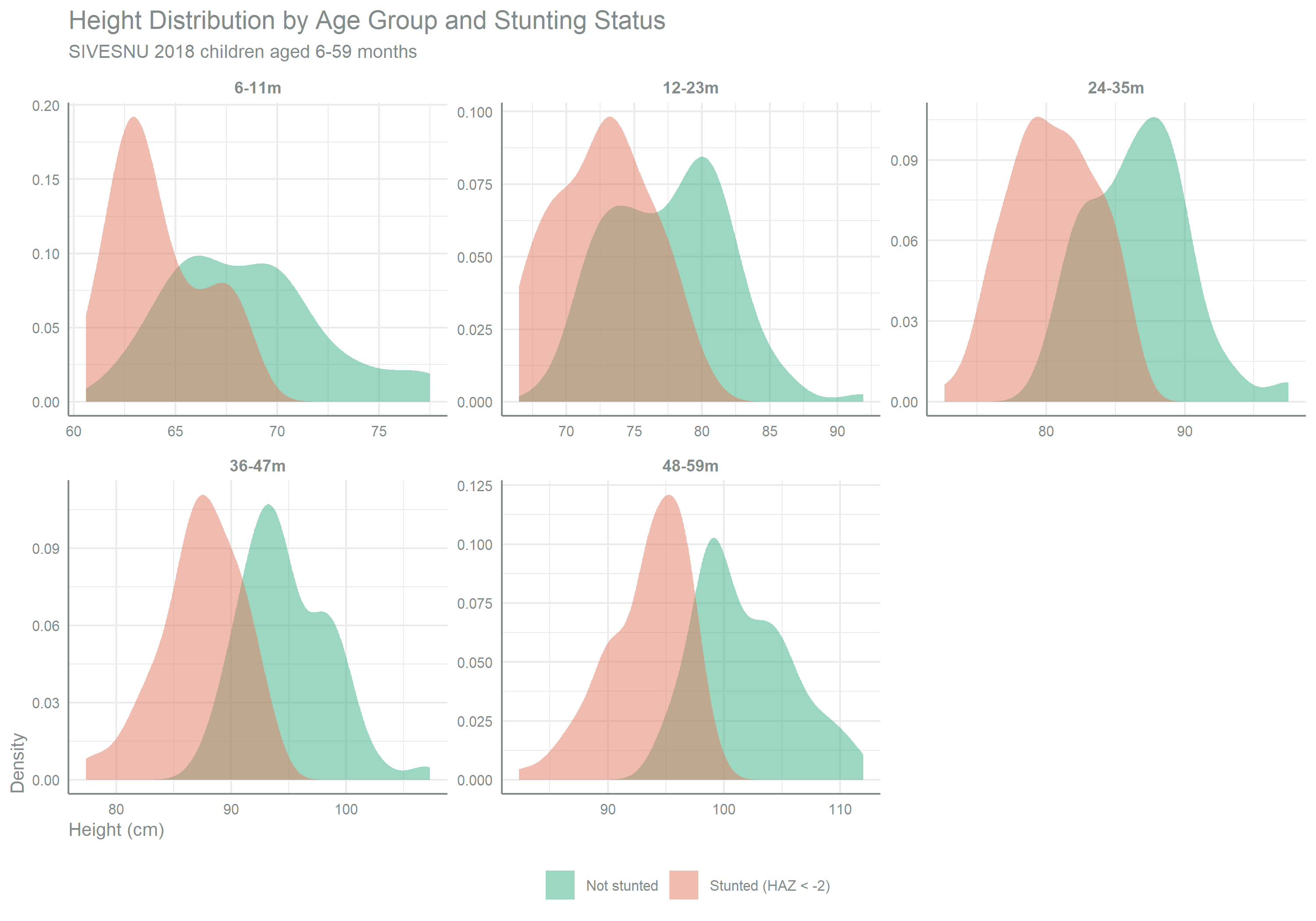
Faceted density plot with one panel per age group, each showing height in centimetres on the x-axis. Within every panel two overlaid curves compare children who are not stunted (green) against those who are stunted with HAZ below -2 (orange). In each age group the stunted curve sits at shorter heights than the not-stunted curve, and both shift rightward with older age groups, with the distance between the two curves widening from the youngest panel to the oldest. — Figure 3: Height distribution by age group and stunting status

The two curves are separated in every age group, and the distance between their means grows from 4.4 cm at 6-11 months to 8.4 cm at 48-59 months. This pattern is consistent with the cumulative character of chronic undernutrition, and it is the signal the transfer model carries into ENCOVI.

Summary

Key Findings

Training dataset: 773 SIVESNU 2018 children aged 6-59 months with valid anthropometric measurements form the training population for the height transfer model.
Variable harmonization: 22 predictor variables are harmonized between the SIVESNU and ENCOVI coding schemes, and every child matches to a household socioeconomic profile.
Data quality: 11 cells are missing across the predictor set, each affected variable below 1% of records, and all of them categorical. They are filled by Random Forest imputation, whose categorical OOB error stands at 0.3171.
Feature selection: 14 of 20 candidate predictors are selected by Boruta. Age leads the importance ranking by an order of magnitude, and geographic and housing indicators form a secondary cluster.

Limitations

SIVESNU sampling bias — SIVESNU 2018 uses a health center-based sampling frame, which may over-represent children who access public health services. The bias is addressed by the weight recalibration against ENSMI stunting prevalence in transferring height to ENCOVI.
Cross-sectional design — Height is measured at a single point in time, so the transfer model estimates the association between socioeconomic profiles and height.
Sample size — 773 children supports the 14 selected predictors, and bounds how much interaction structure the model can resolve, particularly in the smaller departments.
Categorical imputation error — The OOB misclassification rate for the four imputed variables is 0.3171, above the 0.2 reference value.

Application

This modeling-ready dataset, along with the saved transformation objects and the Boruta selection results, feeds the height transfer model, trained on SIVESNU and then applied to ENCOVI 2023 children in transferring height to ENCOVI.