Skip to main content

Generating Synthetic Population

Module 4: Covariate Prediction

Overview

Scenario simulation needs a population that carries three things at once: the demographic and geographic structure of Guatemala, the dietary record of each child, and an anthropometric outcome to move. No single survey carries all three.

ENCOVI 2023 carries the first two. It is nationally representative, it holds the household and geographic attributes that scenario assignment works on, and it records food consumption in enough detail to derive each child’s nutrient intake. What it does not record is child height.

SIVESNU 2018 records height. It provides height-for-age z-scores for children in the same 6–59 month range, but its sample is small and its departmental coverage uneven, so it cannot itself serve as the population of a departmental simulation.

This module builds the simulation population from the ENCOVI side and supplies the missing outcome by statistical matching against SIVESNU:

1. Receptor cohort — Every record is an ENCOVI child aged 6–59 months with a complete dietary record, keeping its household, department and design weight.
2. Bridge model — A model of the height-for-age z-score estimated on the variables both surveys collect, which places donors and receptors on a single comparable metric.
3. Donation — Each receptor is matched to its nearest donors on that metric, within its region and age band, and receives the anthropometric block of one selected donor.
4. Departmental anchoring — Donor selection is tilted, department by department, so that weighted stunting prevalence approaches the Encuesta Nacional de Salud Materno Infantil (ENSMI) 2014–2015 reference (Ministerio de Salud Pública y Asistencia Social et al., 2017).
5. Nutrient profile — Supplementation is added and the derived nutrient variables are recomputed from the child’s own ENCOVI intake.
6. Weight calibration — Design weights are calibrated to that same departmental reference, holding each department’s weighted population fixed.

The resulting dataset is the input to the biofortification scenarios.

Building the Two Cohorts

Receptor Cohort

The receptors are the children the simulation acts on: ENCOVI 2023 children aged 6–59 months with a complete dietary record. Age in months is the value estimated in Estimate Age in Months from the National Statistics Institute (INE) birth registry distributions.

Each receptor keeps its household identifier, its department and its design weight, so the departmental composition of the synthetic population and the joint structure of household, geographic and dietary attributes are those of the survey.

One attribute is completed at this point. Household education is missing for a small number of records and is required later, both as a bridge variable and as a predictor of the nutrient imputation in Baseline and QPM Profiles. Missing values are filled with the weighted median of the child’s own department and area, which keeps the completion inside the cell the variable is used to distinguish.

Table 1: Receptor cohort by department

Receptor Cohort. ENCOVI 2023 children 6-59 months with a complete dietary record

Receptor Cohort
ENCOVI 2023 children 6-59 months with a complete dietary record
	Region	Department	Children	Households	Weighted population
	Central	Chimaltenango	204	170	67,369
	Central	Escuintla	208	178	67,582
	Central	Sacatepéquez	168	146	23,569
	Metropolitana	Guatemala	173	149	182,107
	Noroccidente	Huehuetenango	207	154	151,420
	Noroccidente	Quiché	274	202	163,459
	Nororiente	Chiquimula	136	104	40,513
	Nororiente	El Progreso	138	116	14,541
	Nororiente	Izabal	191	149	42,560
	Nororiente	Zacapa	151	125	22,778
	Norte	Alta Verapaz	247	195	134,646
	Norte	Baja Verapaz	203	159	40,138
	Petén	Petén	200	162	59,218
	Suroccidente	Quetzaltenango	174	145	73,486
	Suroccidente	Retalhuleu	138	121	34,240
	Suroccidente	San Marcos	204	158	125,381
	Suroccidente	Sololá	146	119	41,111
	Suroccidente	Suchitepéquez	223	183	55,686
	Suroccidente	Totonicapán	194	144	53,905
	Suroriente	Jalapa	196	155	45,575
	Suroriente	Jutiapa	173	148	47,234
	Suroriente	Santa Rosa	117	102	36,044
Total	—	—	4,065	3,284	1,522,562

Donor Pool

The donors are the SIVESNU 2018 children carrying a valid height-for-age z-score, together with the variables the matching needs and the anthropometric block that is transferred. Donors are organised by region and age band, which are the cells the matching operates within.

Table 2: Donor pool by region and age band

Donor Pool. SIVESNU 2018 children with a valid height-for-age z-score, by donation cell

Donor Pool
SIVESNU 2018 children with a valid height-for-age z-score, by donation cell
Region	Age band (months)
	[6,12)	[12,24)	[24,36)	[36,60)
Central	13	18	29	50
Metropolitana	11	31	25	71
Noroccidente	13	24	29	50
Nororiente	6	13	6	44
Norte	10	18	15	38
Petén	3	7	10	16
Suroccidente	17	43	36	72
Suroriente	0	9	11	13

NoteAsymmetry Between the Two Cohorts

There are 4,065 receptors and 751 donors, so donors are used by more than one receptor. Donor usage and the reach of the candidate sets are reported in the diagnostics below.

Table 3: Availability of the donated variable block

Donated Block Coverage. Variables transferred from the donor record

Donated Block Coverage
Variables transferred from the donor record
Category	Variables	Available in donor pool
Anthropometric outcome	1	1
Household and child attributes	8	8
Raw transfer-model signal	12	12
Block PCA inputs	123	123

Harmonizing the Bridge Variables

The matching only works if a variable means the same thing on both sides. The bridge variables are therefore brought to a common encoding: factor levels are aligned to a single ordered set, levels observed in fewer than 15 donors are collapsed into a residual category, and the resulting encoding is applied identically to donors and receptors.

Table 4: Bridge variable harmonization

Bridge Variable Harmonization. Level alignment applied identically to donors and receptors

Bridge Variable Harmonization
Level alignment applied identically to donors and receptors
Variable	Levels retained	Levels collapsed	% rare (receptors)	% missing (receptors)	Assigned level	In bridge model
sexo	2	0	0.0	0.0	Hombre	TRUE
area	2	0	0.0	0.0	Rural	TRUE
propiedad	3	2	3.2	0.0	Other	TRUE
tipo_vivienda	2	3	9.0	0.0	Other	TRUE
material_paredes	5	3	5.1	0.0	Other	TRUE
material_techo	5	0	0.1	0.0	Lamina metalica	TRUE
material_piso	4	2	1.0	0.0	Other	TRUE
tipo_sanitario	2	0	0.0	5.8	Uso exclusivo	TRUE
fuente_agua	7	1	0.8	0.0	Other	TRUE
recoleccion_basura	4	0	0.0	5.5	La queman o la entierran	TRUE
electricidad	2	0	0.0	0.0	Si	TRUE
televisor	2	0	0.0	0.0	Si	TRUE
telefonia_celular	2	0	0.0	0.0	Si	TRUE
computadora	2	0	0.0	0.0	No	TRUE

NoteDietary Position

The nutritional index enters the bridge model as the child’s survey-weighted percentile within the intake distribution of its own survey. A percentile is free of the scale of the underlying measurements, which is what lets the dietary dimension inform the matching across two sources whose absolute intake levels are not directly comparable.

The Bridge Model

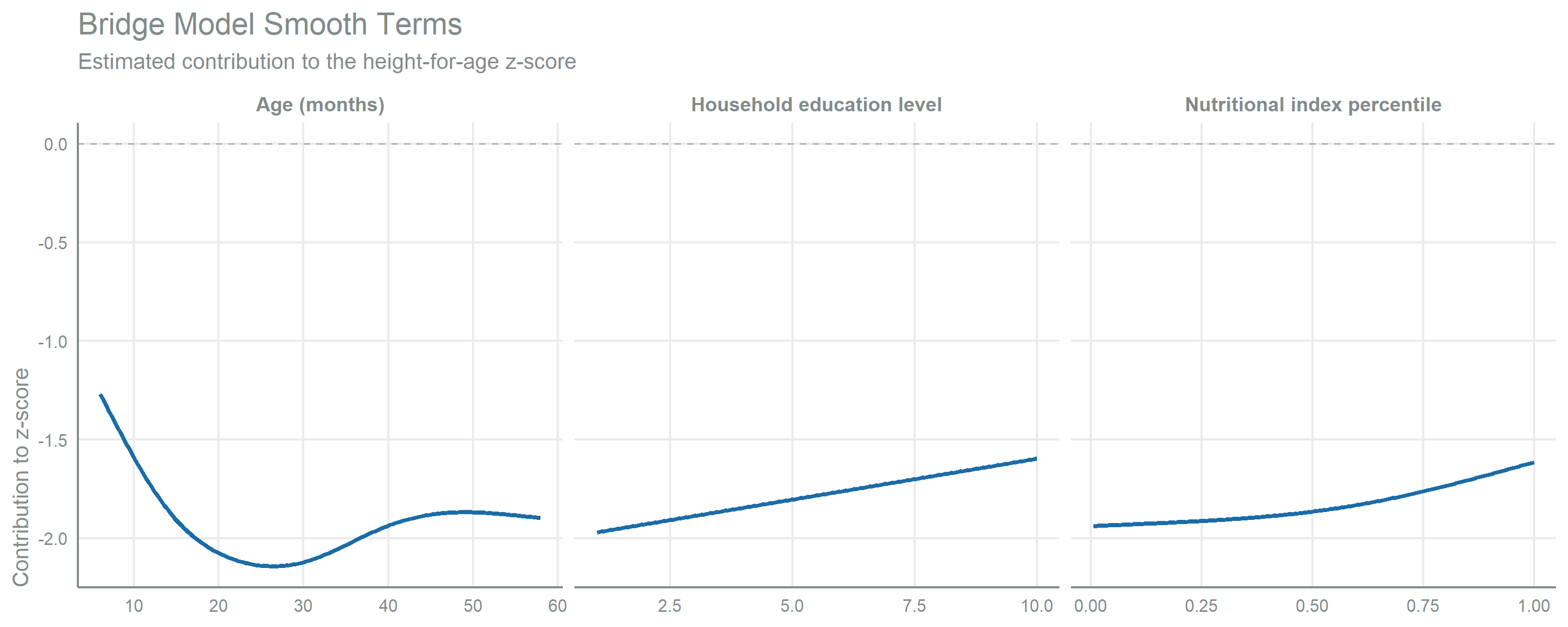
The bridge model relates the height-for-age z-score to the variables both surveys collect. Its purpose is not prediction: it defines a one-dimensional metric on which donors and receptors are comparable. Two children with the same predicted value share the same expected anthropometric position given everything both surveys observe.

Age and the two continuous covariates enter through penalized smooth terms; the harmonized factors enter parametrically.

Table 5: Bridge model fit

Bridge Model. Height-for-age z-score on the variables shared by both surveys

Bridge Model
Height-for-age z-score on the variables shared by both surveys
Metric	Value
Donors	751
Model terms	18
Effective degrees of freedom	49.5
Observations per parameter	15.2
Deviance explained	32.8%
Adjusted R-squared	0.281
Fitted-observed correlation	0.547
Outcome standard deviation	1.226
Residual standard deviation	1.027

Figure 1: Estimated smooth terms of the bridge model

ImportantWhat the Bridge Model Carries

The model accounts for 32.8% of the deviance in the donor pool, with a fitted-observed correlation of 0.547. That is the share of anthropometric position the shared variables locate; the remainder travels across as the selected donor’s residual, described next.

Donation

Candidate Sets and Residual Transfer

Each receptor is matched to the five donors closest to it on the bridge metric, within its donation cell of region and age band. Cells holding fewer donors than the candidate set draw from the full pool, so every receptor is matched.

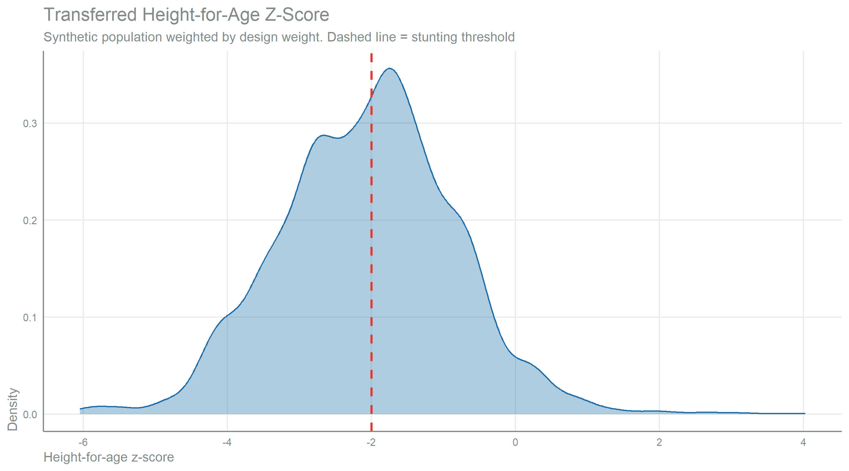
The transferred z-score is the receptor’s own predicted value plus the residual of the selected donor. The predicted component follows the receptor’s characteristics; the residual component reproduces the empirical dispersion of the outcome. Together they retain the variance and shape observed in the donor pool without assuming a parametric error form.

NoteWhy Cells Are Regional

Candidate donors are drawn within region and age band rather than within department. Departmental information reaches the population through the receptor’s own attributes and through the departmental anchoring described next, so the donor pool is asked only for the conditional structure its sample size supports.

Departmental Anchoring

Selection within each candidate set is governed by a departmental parameter that shifts the probability of drawing a donor whose transferred z-score falls below the stunting threshold. The expected weighted prevalence is monotone in that parameter, so the value reproducing the ENSMI reference is unique and is found by root finding.

The magnitude of the parameter is itself informative: it measures how far the departmental level sits from what the shared variables predict on their own.

Table 6: Departmental tilt and achieved prevalence

Departmental Anchoring. Tilt parameter and achieved prevalence against the ENSMI 2014-2015 reference

Departmental Anchoring
Tilt parameter and achieved prevalence against the ENSMI 2014-2015 reference
Department	Children	Achieved	SE (pp)	ENSMI reference	Tilt1	At boundary	Gap (pp)	Gap (SE)2
Alta Verapaz	247	50.1%	3.38	50.0%	−0.46	FALSE	0.08	0.02
Baja Verapaz	203	46.9%	3.78	50.2%	−0.03	FALSE	−3.31	−0.88
Chimaltenango	204	62.7%	3.69	56.5%	−0.32	FALSE	6.23	1.69
Chiquimula	136	54.0%	4.56	55.6%	1.05	FALSE	−1.58	−0.35
El Progreso	138	30.1%	4.20	29.1%	−0.21	FALSE	1.04	0.25
Escuintla	208	23.2%	3.16	26.9%	−1.74	FALSE	−3.69	−1.17
Guatemala	173	26.6%	3.60	25.3%	−2.93	FALSE	1.29	0.36
Huehuetenango	207	71.9%	3.26	67.7%	−0.32	FALSE	4.23	1.30
Izabal	191	28.0%	3.65	26.4%	−0.97	FALSE	1.57	0.43
Jalapa	196	54.5%	3.77	53.8%	0.52	FALSE	0.68	0.18
Jutiapa	173	39.2%	4.37	35.7%	−0.30	FALSE	3.51	0.80
Petén	200	36.6%	3.66	36.1%	0.71	FALSE	0.54	0.15
Quetzaltenango	174	50.6%	4.07	48.8%	0.48	FALSE	1.80	0.44
Quiché	274	71.9%	2.94	68.7%	−0.20	FALSE	3.19	1.08
Retalhuleu	138	30.3%	4.28	34.2%	−0.91	FALSE	−3.88	−0.91
Sacatepéquez	168	46.2%	4.09	42.4%	−0.32	FALSE	3.83	0.94
San Marcos	204	57.5%	3.73	54.8%	−0.12	FALSE	2.66	0.71
Santa Rosa	117	33.3%	4.67	33.6%	−0.74	FALSE	−0.35	−0.07
Sololá	146	64.4%	4.18	65.6%	1.28	FALSE	−1.21	−0.29
Suchitepéquez	223	37.2%	3.49	39.6%	−0.46	FALSE	−2.39	−0.68
Totonicapán	194	69.0%	3.55	70.0%	1.01	FALSE	−1.05	−0.30
Zacapa	151	39.5%	4.11	40.0%	0.02	FALSE	−0.55	−0.13
1 Tilt is the departmental parameter governing donor selection, searched within the range -8 to 8. A value at the boundary would mean the reference could not be reached within that range.
2 Gap (SE) expresses the departure from the reference in units of its own standard error.

TipAnchoring Result

After the tilt, departmental prevalence departs from the ENSMI reference by 2.21 percentage points on average and by 6.23 at the widest departure, with 18 of the 22 departments inside one standard error. No department reaches the boundary of the admissible tilt range.

The tilt sets prevalence in expectation, over the random draw of donors. The weight calibration below fixes it on the realised sample.

Donation Diagnostics

Because the donor pool is smaller than the receptor cohort, how often each donor is reused and how far the candidate sets reach are properties worth reporting.

Table 7: Donor usage and matching distance by region

Donor Usage. Reuse and matching distance within each region

Donor Usage
Reuse and matching distance within each region
Region	Receptors	Donors used	Max reuse	Median reuse	Top donor (% weighted)	Mean distance	% from own cell
Central	580	90	24	5.00	4.3	0.13	100.0
Metropolitana	173	62	15	2.00	9.0	0.20	100.0
Noroccidente	481	106	12	4.00	2.1	0.10	100.0
Nororiente	616	65	33	8.00	6.1	0.37	100.0
Norte	450	78	15	5.00	2.7	0.14	100.0
Petén	200	35	15	6.00	8.4	0.27	100.0
Suroccidente	1,079	155	35	6.00	3.7	0.09	100.0
Suroriente	486	32	46	11.50	9.8	0.34	90.3

Table 8: Transferred z-score distribution against the donor pool

Transferred Distribution. Survey-weighted on the scale of each source

Transferred Distribution
Survey-weighted on the scale of each source
Statistic	Donor pool	Synthetic population
Mean	−1.89	−2.05
SD	1.23	1.21
P5	−3.92	−4.04
P25	−2.70	−2.84
P50	−1.88	−2.00
P75	−1.09	−1.27
P95	0.09	−0.17

Figure 2: Transferred height-for-age z-score distribution

Nutrient Profile

Supplementation Contribution

The micronutrient powder programme delivers iron and zinc through daily sachets. Its expected contribution is added to the non-maize component of each child’s intake, scaled by the departmental coverage published by INE and by a national adherence factor of 0.719. That factor is the survey-weighted mean of the adherence estimated in Chispitas Supplementation, taken over the SIVESNU 2018 children recorded as programme recipients, which is the full set of recipients in that survey rather than the subset selected as donors.

Table 9: Expected supplementation contribution by department

Chispitas Contribution. Expected daily addition to non-maize iron and zinc | Adherence among recipients: 0.719

Chispitas Contribution
Expected daily addition to non-maize iron and zinc | Adherence among recipients: 0.719
Department	Coverage	Iron (mg/day)	Zinc (mg/day)
Sololá	91.0%	2.180	0.894
Chiquimula	86.2%	2.065	0.847
Chimaltenango	84.8%	2.032	0.833
Jutiapa	82.1%	1.967	0.807
Petén	79.3%	1.900	0.779
Sacatepéquez	77.8%	1.864	0.764
Escuintla	77.5%	1.857	0.761
Totonicapán	76.3%	1.828	0.750
Alta Verapaz	71.7%	1.718	0.704
Santa Rosa	71.5%	1.713	0.702
El Progreso	69.5%	1.665	0.683
Baja Verapaz	68.1%	1.632	0.669
Jalapa	63.7%	1.526	0.626
Retalhuleu	61.6%	1.476	0.605
Quiché	61.5%	1.474	0.604
Quetzaltenango	56.8%	1.361	0.558
Zacapa	53.0%	1.270	0.521
Suchitepéquez	48.3%	1.157	0.474
Huehuetenango	45.4%	1.088	0.446
San Marcos	39.9%	0.956	0.392
Guatemala	36.3%	0.870	0.357
Izabal	20.9%	0.501	0.205

Derived Variables

Total intake, absorbed fractions and the composite nutritional index are computed from the source-specific components of the child’s own ENCOVI record. Iron absorption uses the fixed fraction adopted for predominantly plant-based diets and zinc absorption follows the Miller saturation model with its age term, as documented in Bioavailability Adjustments.

The derivation runs twice:

• The whole-diet pass uses maize and non-maize together and produces the descriptive nutrient profile of the synthetic population.
• The non-maize pass uses only the non-maize sources and produces the index at which the GAM effect model is evaluated. It applies the Miller model to the non-maize zinc pool alone and uses its own normalization parameters.

The absorption constants are identical in both passes, so the axis the effect model was estimated on and the axis it is evaluated on are constructed the same way.

Table 10: Nutrient profile of the synthetic population

Nutrient Profile. Synthetic population after supplementation and derivation

Nutrient Profile
Synthetic population after supplementation and derivation
Variable	Mean	P25	Median	P75
fe_mg_total	15.51	6.01	9.95	16.93
zn_mg_total	10.24	3.22	5.79	10.78
prot_g_total	25.03	8.97	16.26	28.47
lys_mg_total	1.83	0.68	1.24	2.08
trp_mg_total	0.39	0.13	0.24	0.43
ene_kcal_total	1,690.61	532.40	981.44	1,811.00
fe_absorbed_mg	0.78	0.30	0.50	0.85
taz_mg	1.17	0.83	1.18	1.51
nutritional_index	0.42	−0.52	−0.03	0.67

Block Components

The block components the response model references are recomputed from the donated variables using the transformations fitted in Stunting Modeling Data.

Table 11: Block PCA components carried into the synthetic population

Block PCA Components. Transformations applied to the donated variables

Block PCA Components
Transformations applied to the donated variables
Block	Description	Input variables	Components
child_controls	Child health check-ups	13	5
child_development	Child development milestones	25	7
chispitas	Chispitas supplementation behavior	12	4
dental_child	Child dental health	14	6
fortification	Fortified food consumption	34	13
wealth	Household wealth indicators	25	8

Weight Calibration

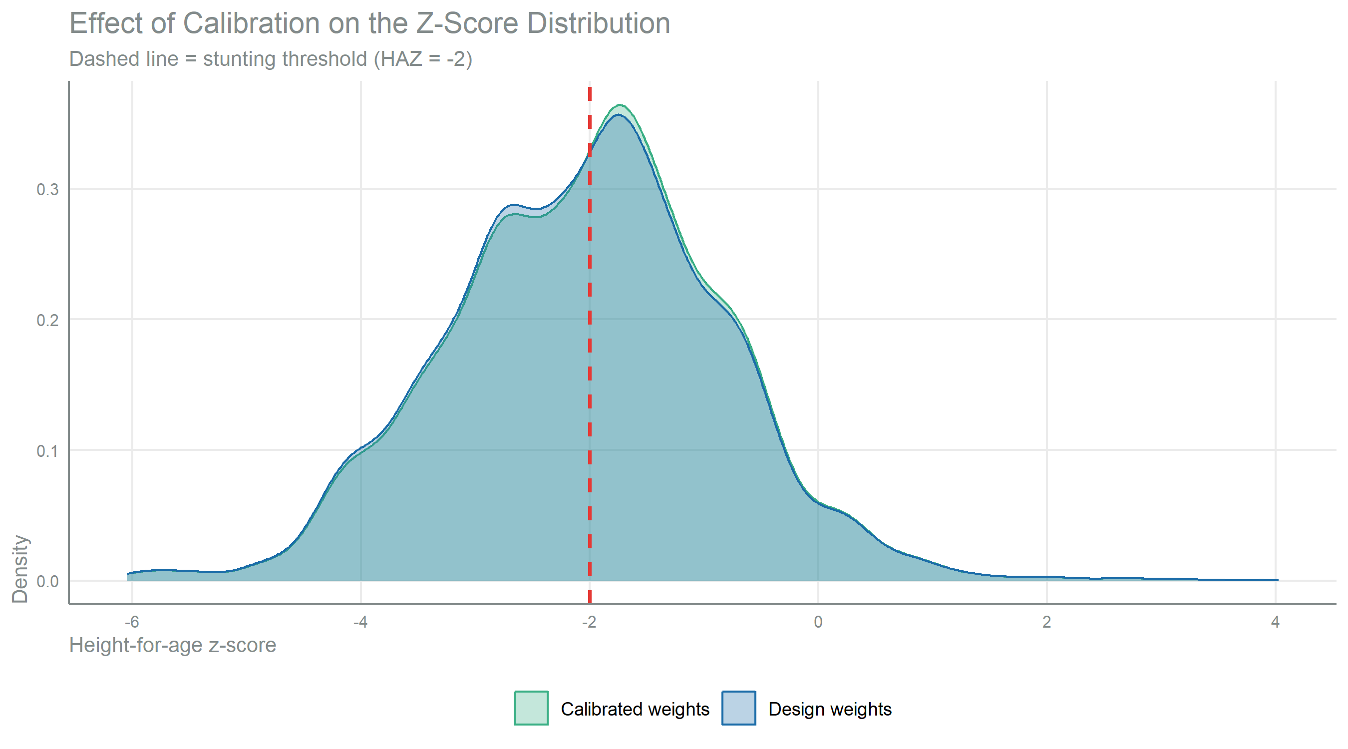
Design weights are calibrated so that weighted departmental prevalence reproduces the ENSMI reference, holding each department’s weighted population total fixed.

Table 12: Weight calibration diagnostics

Calibration Diagnostics. Effect of the calibration on the weight distribution

Calibration Diagnostics
Effect of the calibration on the weight distribution
Metric	Value
Weight CV (design)	73.5%
Weight CV (calibrated)	73.8%
Design effect	1.545
Adjustment ratio range	[0.9, 1.17]
Ratios outside [0.5, 2.0]	0.0%
Maximum covariate shift	0.15%

TipScale of the Adjustment

Individual weights move within a ratio range of [0.9, 1.17], and the largest shift induced in any covariate mean is 0.15%. The calibration reaches the departmental targets without displacing the composition of the population it acts on.

Table 13: Departmental prevalence after calibration

Calibration Results. Weighted prevalence by department against the ENSMI reference

Calibration Results
Weighted prevalence by department against the ENSMI reference
Department	Children	Weighted population	Prevalence	Mean z-score	ENSMI reference	Gap (pp)
Alta Verapaz	247	134,646	50.0%	−2.05	50.0%	0.00
Baja Verapaz	203	40,138	50.2%	−1.96	50.2%	0.00
Chimaltenango	204	67,369	56.5%	−2.13	56.5%	0.00
Chiquimula	136	40,513	55.6%	−1.67	55.6%	0.00
El Progreso	138	14,541	29.1%	−1.26	29.1%	0.00
Escuintla	208	67,582	26.9%	−1.53	26.9%	0.00
Guatemala	173	182,107	25.3%	−1.63	25.3%	0.00
Huehuetenango	207	151,420	67.7%	−2.55	67.7%	0.00
Izabal	191	42,560	26.4%	−1.44	26.4%	0.00
Jalapa	196	45,575	53.8%	−2.12	53.8%	0.00
Jutiapa	173	47,234	35.7%	−1.65	35.7%	0.00
Petén	200	59,218	36.1%	−1.56	36.1%	0.00
Quetzaltenango	174	73,486	48.8%	−2.13	48.8%	0.00
Quiché	274	163,459	68.7%	−2.46	68.7%	0.00
Retalhuleu	138	34,240	34.2%	−1.90	34.2%	0.00
Sacatepéquez	168	23,569	42.4%	−1.77	42.4%	0.00
San Marcos	204	125,381	54.8%	−2.29	54.8%	0.00
Santa Rosa	117	36,044	33.6%	−1.61	33.6%	0.00
Sololá	146	41,111	65.6%	−2.33	65.6%	0.00
Suchitepéquez	223	55,686	39.6%	−2.03	39.6%	0.00
Totonicapán	194	53,905	70.0%	−2.49	70.0%	0.00
Zacapa	151	22,778	40.0%	−1.48	40.0%	0.00

Table 14: Z-score distribution under design and calibrated weights

Distributional Effect of the Calibration. Donor pool, design weights and calibrated weights

Distributional Effect of the Calibration
Donor pool, design weights and calibrated weights
Statistic	Donor pool	Design weights	Calibrated weights
Mean	−1.89	−2.05	−2.03
SD	1.22	1.21	1.21
Prevalence	0.45	0.50	0.49
P5	−3.92	−4.04	−4.03
P25	−2.70	−2.84	−2.83
P50	−1.88	−2.00	−1.97
P75	−1.09	−1.27	−1.26
P95	0.09	−0.17	−0.15

Figure 3: Z-score density under design and calibrated weights

Output

Table 15: Variable inventory of the synthetic population

Output Inventory. Variables carried by the synthetic population dataset

Output Inventory
Variables carried by the synthetic population dataset
	Category	Variables	Source
	Identifiers and weights	3	Receptor cohort and calibration
	Survey context	5	Receptor cohort
	Dietary components	13	ENCOVI 2023
	Derived nutritional variables	11	Computed in Phase E
	ENCOVI household record	3	ENCOVI 2023
	Donated attributes	8	Donor transfer
	Raw signal + non-maize axis	15	Donor transfer + Phase E
	Block components	12	Computed in Phase F
	Anthropometric outcome	2	Donor transfer
Total	—	72	—

Summary

Key Findings

1. Bridge model coverage: The variables shared by both surveys account for 32.8% of the deviance in the donor pool, with a fitted-observed correlation of 0.547. The rest of each child’s anthropometric position travels across as the selected donor’s residual.

2. Departmental anchoring: After the tilt, weighted departmental prevalence departs from the ENSMI reference by 2.21 percentage points on average, with 18 of 22 departments inside one standard error and none at the boundary of the admissible range.

3. Calibration closes the residual gap: After weight calibration the departmental gap is 0 percentage points at its widest, with adjustment ratios inside [0.9, 1.17] and a largest covariate mean shift of 0.15%.

4. Output: 4,065 children across 3,284 households, representing 1,522,562 children nationally, carrying 72 variables.

WarningLimitations

1. Conditional independence — The donation assumes that, given the shared variables, the anthropometric block is independent of the variables observed only in ENCOVI. This assumption is not verifiable from the data.

2. Donor reuse — The donor pool is smaller than the receptor cohort, so donors are used by more than one receptor. Usage and mean matching distance are reported by region.

3. Reference period — The departmental reference predates the receptor survey. The departmental anchoring absorbs changes in level occurring between the two collection periods.

Application

This population is the input to Baseline and QPM Profiles, which computes each child’s baseline and biofortified nutrient profile, and through it to the scenario simulation.

References

Ministerio de Salud Pública y Asistencia Social, Instituto Nacional de Estadística, & ICF International. (2017). Encuesta Nacional de Salud Materno Infantil 2014-2015. Informe Final. MSPAS/INE/ICF.