Applying Transfer Models to SIVESNU

Module 4: Covariate Prediction

Overview

The transfer models developed in Module 3 enable us to predict nutrient intake for populations where detailed food consumption data is unavailable. SIVESNU 2018 (Sistema de Vigilancia Epidemiológica de Salud y Nutrición) provides anthropometric measurements and food security indicators for Guatemalan children, but lacks the detailed dietary recall needed to calculate nutrient intake directly.

By applying our ENCOVI-trained models to the SIVESNU data, we can:

Estimate individual nutrient intake — Predict iron, zinc, protein, lysine, tryptophan, and energy intake for each child based on their demographic and socioeconomic characteristics.
Link nutrition to stunting outcomes — Connect predicted intake with measured height-for-age z-scores to model the nutrition–stunting relationship.
Enable biofortification simulation — Create a baseline for comparing conventional vs. biofortified maize scenarios.

This module bridges the gap between ENCOVI’s food consumption data and SIVESNU’s anthropometric measurements, creating a unified analytical dataset for impact modeling.

Data Sources

SIVESNU 2018

SIVESNU is Guatemala’s national nutrition surveillance system, collecting data on child health and nutritional status (Instituto de Nutrición de Centro América y Panamá, 2020). The 2018 round provides:

Anthropometric data — Height-for-age z-scores for children 6–59 months.
Household characteristics — Socioeconomic indicators matching ENCOVI structure.
Food security assessment — FIES (Food Insecurity Experience Scale) responses.

SIVESNU does not include the detailed food consumption records that ENCOVI carries, so nutrient intake cannot be calculated directly from it. This is the gap the transfer models address.

ENCOVI Reference Distributions

To calibrate our predictions, we use the observed nutrient distributions from ENCOVI 2023 as reference targets, restricted to children aged 6–59 months so that the reference describes the same population as the target. Quantile mapping transports the predicted SIVESNU distributions onto the empirical patterns of that reference.

Nutrient intake scales with body size, and the ENCOVI children in this age range consume roughly half of what the all-age population does — median ratios of 0.57 for the maize-source components and 0.47–0.49 for the non-maize components. Restricting the reference to the same age range keeps both the level and the composition of the calibrated values on the child scale.

Transfer Models

The 13 gamma regression models from Module 3 predict nutrient intake separately for maize and non-maize sources. This separation enables biofortification simulation by modifying only the maize component while preserving baseline non-maize intake.

Variable Harmonization

Aligning Survey Structures

SIVESNU and ENCOVI use different variable names and coding schemes for similar concepts. Before applying transfer models, we must harmonize SIVESNU variables to match the exact structure expected by the ENCOVI-trained models.

This harmonization includes:

Factor level alignment — Ensuring categorical variables have identical levels and ordering.
Variable renaming — Matching ENCOVI naming conventions.
Derived variables — Creating composite indicators (e.g., household parental education level) using the same methodology.

Missing Value Imputation

Survey data inevitably contains missing values. We apply Random Forest-based multivariate imputation because it:

Handles mixed data types (continuous and categorical) simultaneously.
Preserves variable correlations and multivariate structure.
Provides out-of-bag error estimates for quality assessment.

Implementation uses the impute_rf_parallel() utility function, which wraps missRanger with a multi-threaded ranger engine and returns imputed values alongside out-of-bag error estimates (OOBE for continuous variables, PFC for categorical). The multi-threaded engine accelerates the iterative imputation process without altering the underlying methodology, which remains the standard chained Random Forest approach.

About out-of-bag error

Out-of-bag (OOB) error estimates are calculated from observations that were randomly excluded during tree construction within the Random Forest algorithm, providing an internal quality metric for imputed values without requiring a separate test set.

Table 1: Random Forest imputation quality metrics

Missing Value Imputation Quality Assessment. Out-of-bag error estimates from Random Forest imputation (includes FIES variables)
Metric	Value	Quality Assessment
Missing Value Imputation Quality Assessment
Out-of-bag error estimates from Random Forest imputation (includes FIES variables)
OOBE (Continuous Variables)¹	0.2622	Acceptable
PFC (Categorical Variables)²	0.0423	Acceptable
Number of Iterations	10.0000	Fixed parameter
Trees per Iteration	100.0000	Fixed parameter
¹ OOBE: aggregated out-of-bag error across the continuous variables imputed, bounded in [0, 1] and invariant to their scale. Values < 0.5 indicate acceptable imputation quality for continuous variables.
² PFC: Proportion of Falsely Classified entries. Values < 0.2 indicate acceptable imputation quality for categorical variables.

Imputation Quality

OOBE < 0.5 and PFC < 0.2 are the ranges conventionally treated as acceptable for this imputation method.

Completion of Residual Missing Values

The Random Forest imputation engine can leave a residual NaN for a small subset of rows when the out-of-bag prediction collapses inside a terminal node with zero within-leaf variance. This affects continuous discrete-scale predictors.

Downstream analyses (Yeo-Johnson transformation, model prediction, quantile mapping) operate on a complete predictor matrix, so residual missing values are completed with a variable-specific rule:

Numeric / integer variables: median of the observed values, which preserves the support of discrete-scale ordinal variables (e.g. years of schooling take values such as 1, 1.5, 2, 2.5, …).
Factor variables: mode of the observed values.

Completing rather than discarding keeps every record in the predicted distributions. The count of values completed by each rule is reported in the table below.

Table 2: Residual missing value completion after Random Forest imputation

Residual Missing Value Completion. Values completed by variable-specific rule after RF imputation
Variable	N Completed	Completion Rule
Residual Missing Value Completion
Values completed by variable-specific rule after RF imputation
— Residual NAs after completion —	0	Integrity check: passed

Applying Transformations

Yeo-Johnson Normalization

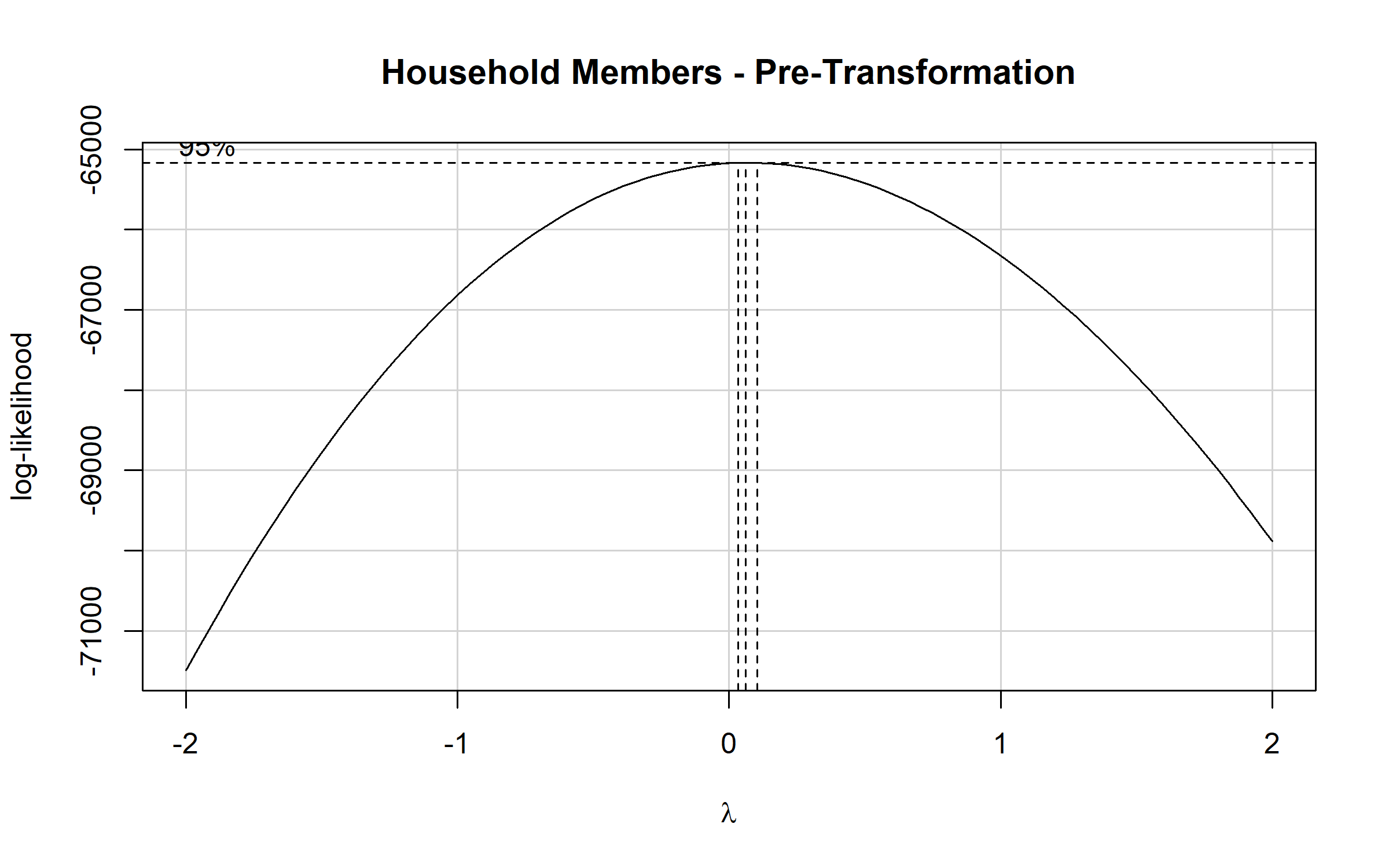
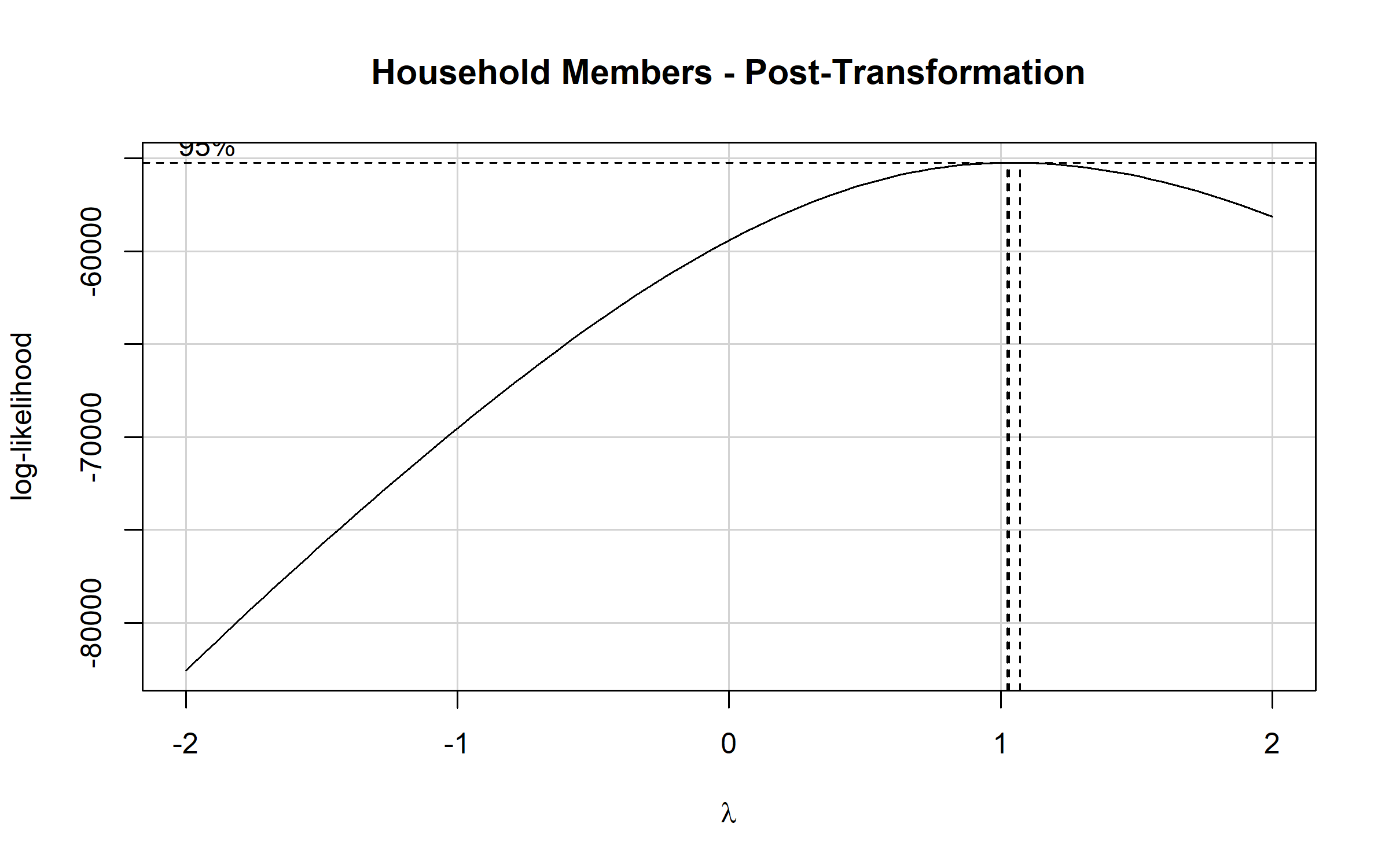
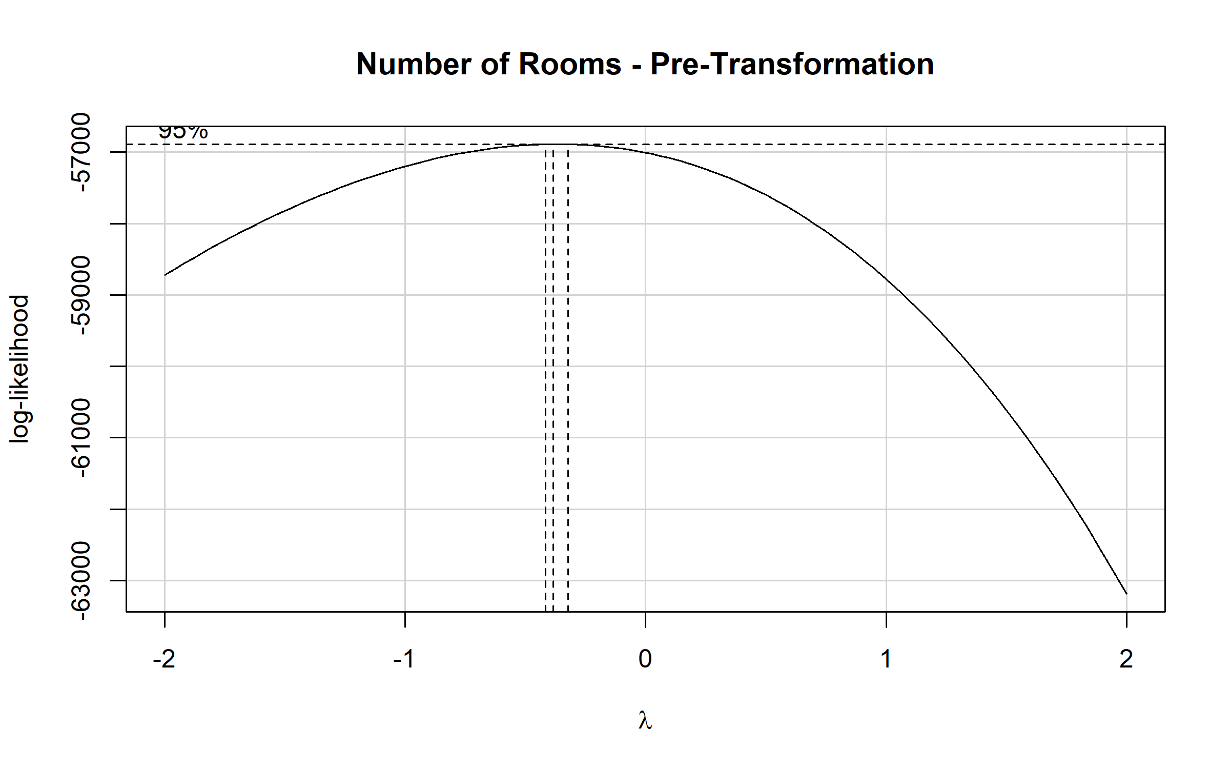
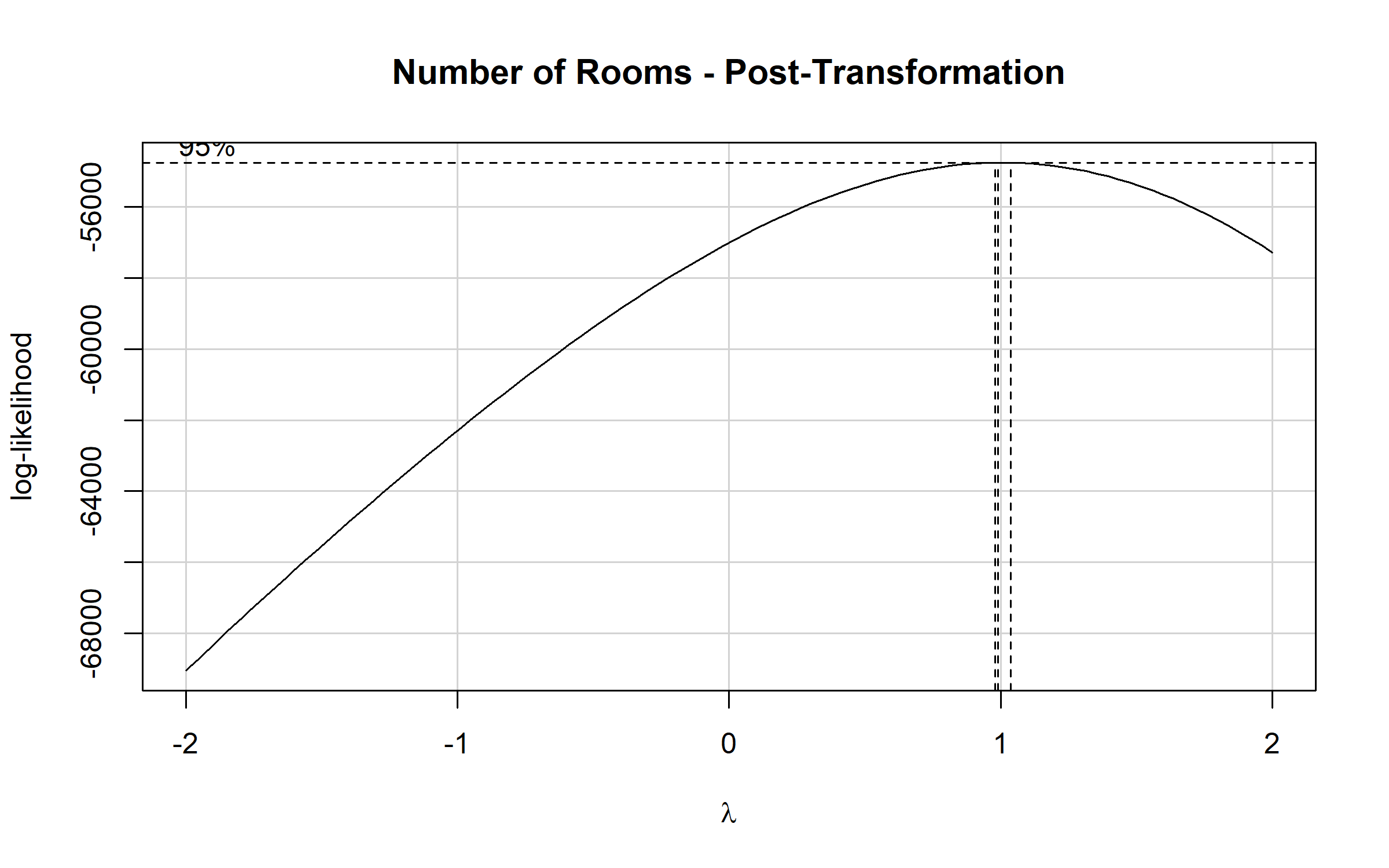
The transfer models were trained on Yeo-Johnson transformed continuous predictors. We apply the same transformations (using parameters fitted on ENCOVI) to ensure SIVESNU data enters the models in the expected scale.

Figure 1: Yeo-Johnson transformation profile for household members (pre-transformation)

Figure 2: Yeo-Johnson transformation profile for household members (post-transformation)

Figure 3: Yeo-Johnson transformation profile for number of rooms (pre-transformation)

Figure 4: Yeo-Johnson transformation profile for number of rooms (post-transformation)

Nutrient Prediction

Model Application

Each transfer model predicts nutrient intake on the log scale (via log link in gamma regression). We apply exponential back-transformation to obtain predictions in natural units (mg/day or g/day).

Link Functions

All nutrient models use log link, so their predictions require exponential back-transformation.

Food Security Adjustment

SIVESNU includes the Food Insecurity Experience Scale (FIES), an 8-question instrument measuring household food security. FIES scores are used to apply a fine adjustment to nutrient intake predictions before quantile mapping:

FIES Score	Food Security Status	Description	Adjustment
0	Food secure	Adequate food access	+5%
1–3	Mild food insecurity	Slight decrease in quantity and/or quality of food consumed	+2%
4–6	Moderate food insecurity	Moderate reduction in quantity and/or quality of food consumed	−2%
7–8	Severe food insecurity	Have run out of food for a day or more	−5%

Why the adjustment is applied. The transfer models predict nutrient intake from demographic and socioeconomic characteristics. Two children sharing the same socioeconomic profile therefore receive identical predicted intake values, regardless of differences in their actual food security situation. Quantile mapping alone cannot separate these two children, because it preserves the ranks it receives — if the inputs are identical, the outputs remain identical.

FIES is used as an independent proxy for the household food environment. Children in more food-insecure households start from a slightly lower intake value (−2% or −5%) than children in more food-secure households (+2% or +5%), even when the transfer model assigned them the same starting point. The adjustment is applied before quantile mapping, so that the subsequent rank-based calibration operates on already-differentiated values rather than on identical ones.

Origin of the adjustment factors. The factors (+5% / +2% / −2% / −5%) are a modeling parameter of this framework. They were set by inspecting the plausible intake distributions across food security strata and choosing modest, symmetric adjustments that introduce the intended differentiation without distorting the overall distribution.

Validation. What is validated is the final intake distribution, after the FIES adjustment, the quantile mapping and the maize-source alignment have all been applied, against the age-matched ENCOVI reference. That comparison is reported at the end of this page.

Role of the Adjustment

The FIES adjustment is a fine-tuning step that introduces a food-security gradient into predictions otherwise driven only by demographic and socioeconomic covariates. Its modest magnitude (at most ±5%) reflects this secondary, corrective role. Its purpose is to improve discrimination between children with similar socioeconomic profiles but different food security status, while avoiding the circularity of using the stunting outcome as an input.

Target Population Filtering

The stunting analysis focuses on children aged 6–59 months, the standard window for assessing chronic malnutrition. Prediction runs on all SIVESNU individuals, and the filter to this age range is applied before the calibration step that follows.

The order matters. Quantile mapping transports the quantiles of a source distribution onto those of a reference, so the two need to describe comparable populations. Filtering first leaves the source on the child scale, matching the ENCOVI reference that was already restricted to the same age range.

Quantile Mapping Calibration

Model predictions do not match the observed ENCOVI distributions exactly. Quantile mapping aligns the predicted distribution to the reference distribution, preserving ranks while correcting systematic level differences. The mapping is estimated over the pooled age-matched range.

Maize-Source Alignment

A rank-based alignment is then applied to the maize-source variables, which realigns each individual’s maize-source values against their overall non-maize nutrient profile.

Assumption Behind the Alignment

The alignment rests on intra-individual nutrient coherence: an individual’s maize-source intake is expected to sit consistently with the rest of their nutrient profile. Maize dependency is itself a marker of household resources, so before the alignment the maize-source block and the stunting outcome share that socioeconomic gradient.

Preserved Raw Predictions

The exported dataset carries two parallel blocks of the twelve source-specific nutrient variables. The _raw block holds the transfer-model output before the FIES adjustment, the quantile mapping and the maize-source alignment; the adjusted block holds the calibrated values that the rest of the pipeline consumes. Each raw column pairs one-to-one with its calibrated counterpart. The raw block is carried unchanged through the remaining scripts of this module and takes no part in any calculation: it exists so that the effect of the calibration can be audited at any stage.

Final Dataset

Variable Selection

The final dataset contains all variables needed for stunting modeling and biofortification scenario simulation.

Table 3: Final dataset structure

Final Dataset Structure. SIVESNU 2018 with predicted nutrient intake values
Variable Category	N Variables	N Observations
Final Dataset Structure
SIVESNU 2018 with predicted nutrient intake values
Identifiers	3	978
Demographics	4	978
Geographic	2	978
Household characteristics	8	978
Basic services	4	978
Household assets	5	978
Food security (FIES)	9	978
Nutritional (raw predictions)	12	978
Nutritional (adjusted)	12	978
Other	1	978
TOTAL	61	978

Distribution Validation Against the Reference

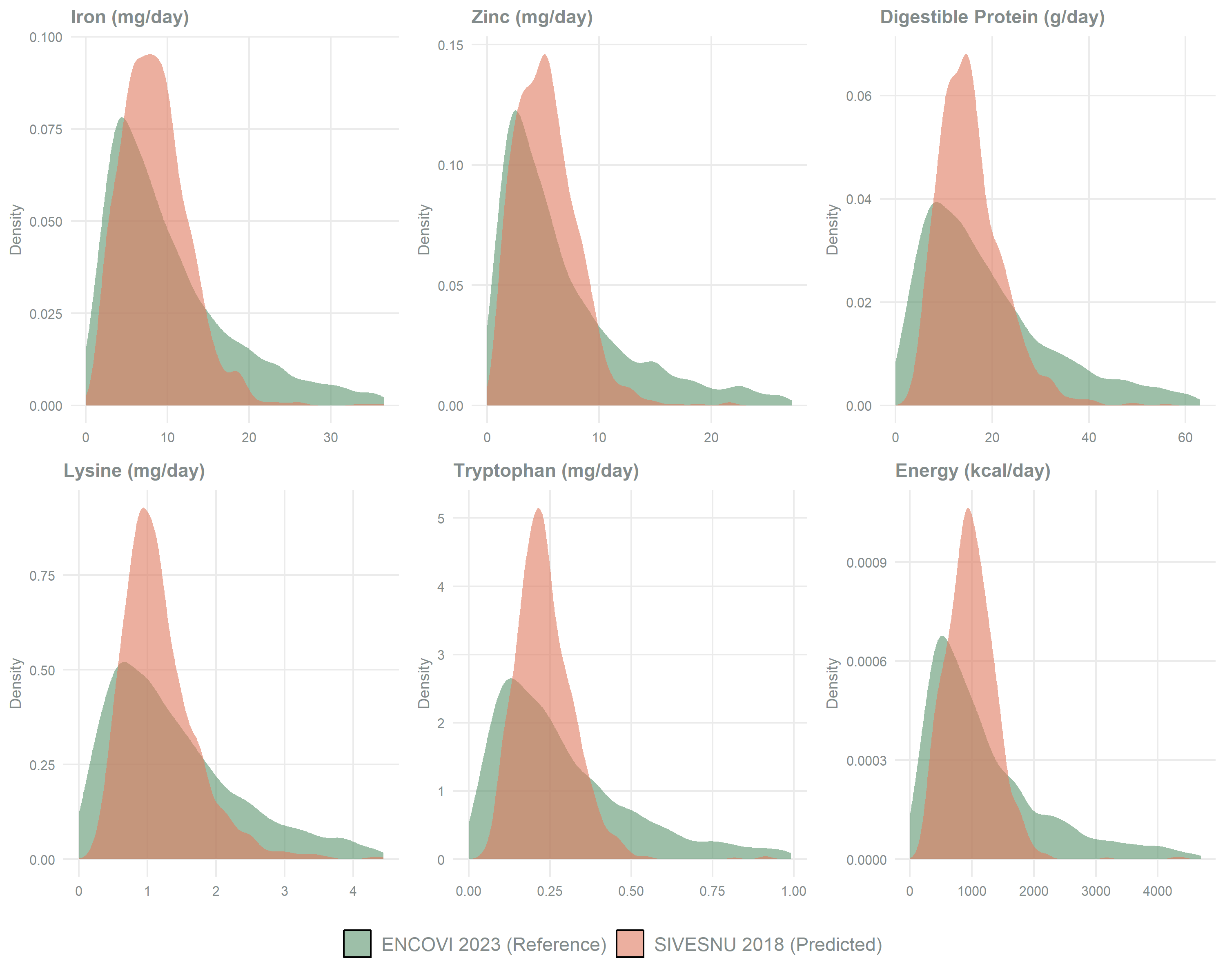
The figure and table below compare the distribution of calibrated nutrient intakes for SIVESNU children (6–59 months) against the ENCOVI children they were mapped onto. Both sides cover the same age range, so this is a like-for-like comparison.

The figure compares total intake per nutrient, where the two populations track each other closely (median ratios between 0.90 and 1.00). The table separates the two source blocks, which behave differently by construction: the non-maize components leave the quantile mapping untouched and sit within 3–8% of the reference medians, with Kolmogorov-Smirnov statistics below 0.075, while the maize-source components sit 14–20% above the reference medians, being the only block modified after the mapping by the rank-based alignment described above.

Grid of six overlaid density plots, one panel per nutrient: iron, zinc, digestible protein, lysine, tryptophan, and energy, each with intake on the x-axis and density on the y-axis. Two filled curves per panel compare the age-matched ENCOVI 2023 children's reference against the SIVESNU 2018 calibrated children's intakes. The paired curves overlap closely in every panel, with the SIVESNU curves sitting marginally lower for digestible protein and lysine. — Figure 5: Distribution comparison: SIVESNU children (6-59m, calibrated) vs ENCOVI children (6-59m, observed)

Table 4: Distribution comparison by source block: SIVESNU children (6-59m) vs age-matched ENCOVI children

Nutrient Intake Distributions — Children 6-59 months, SIVESNU vs ENCOVI. Medians and Kolmogorov-Smirnov statistic against the age-matched calibration reference
Nutrient	From Maize					From Non-Maize
Nutrient Intake Distributions — Children 6-59 months, SIVESNU vs ENCOVI
Medians and Kolmogorov-Smirnov statistic against the age-matched calibration reference
Nutrient	ENCOVI	SIVESNU	Ratio¹	KS²	p-value	ENCOVI	SIVESNU	Ratio	KS	p-value
Iron (mg/day)	3.2	3.7	1.14	0.167	< 0.001	3.7	3.6	0.96	0.067	< 0.01
Zinc (mg/day)	2.6	3.1	1.16	0.170	< 0.001	1.6	1.5	0.92	0.066	< 0.01
Digestible Protein (g/day)	5.1	6.1	1.20	0.179	< 0.001	7.8	7.3	0.94	0.074	< 0.001
Lysine (mg/day)	0.3	0.4	1.19	0.179	< 0.001	0.6	0.6	0.97	0.055	< 0.05
Tryptophan (mg/day)	0.1	0.1	1.19	0.179	< 0.001	0.1	0.1	0.96	0.061	< 0.01
Energy (kcal/day)	436.3	513.6	1.18	0.176	< 0.001	391.9	364.6	0.93	0.053	< 0.05
¹ Ratio = SIVESNU median / ENCOVI median, both for children 6-59 months. Green marks ratios within 0.9 to 1.1. The maize-source block sits above that band because the rank-based alignment is applied after the quantile mapping.
² KS: Kolmogorov-Smirnov statistic on the distribution shape. Green marks values below 0.1.

Reading the Validation

Both sides of the comparison are children aged 6–59 months, so the medians and the Kolmogorov-Smirnov statistics measure how closely the calibrated SIVESNU distributions reproduce the reference they were mapped onto.

The non-maize block is the one that reaches the reference directly: its ratios fall inside the 0.9–1.1 band and its Kolmogorov-Smirnov statistics stay below 0.1. The maize-source block is realigned after the mapping, so its ratios sit above that band by design.

Summary

Processing Pipeline

Step	Method	Purpose
Variable harmonization	Factor recoding	Match ENCOVI predictor structure
Missing imputation	Random Forest (`impute_rf_parallel`)	Handle incomplete records
Residual completion	Median / mode	Complete the predictor matrix
Transformation	Yeo-Johnson	Normalize continuous predictors
Prediction	Gamma GLM	Estimate nutrient intake
Target population filter	Children 6–59 months	Match the age range of the reference
FIES adjustment	Score-based scaling	Incorporate food security
Quantile mapping	Distribution alignment	Calibrate to the age-matched ENCOVI reference
Maize-source alignment	Rank-based realignment	Place the maize block on the individual’s nutrient profile

Key Findings

Age-matched calibration — With the target population filtered before the mapping and the reference restricted to the same age range, the non-maize block reproduces the reference medians within 3–8%, with Kolmogorov-Smirnov statistics below 0.075.
Maize block offset by design — The maize-source components sit 14–20% above the reference medians, the footprint of the rank-based alignment applied after the mapping.
Food security differentiation — The FIES adjustment separates children whose demographic and socioeconomic profiles are identical, which the transfer models alone map to the same predicted intake.

Application

This dataset provides the nutrient intake foundation for:

Chispitas integration — Adding micronutrient supplementation effects.
Bioavailability calculations — Converting intake to absorbed nutrients.
Stunting model development — Linking intake to HAZ outcomes.
Scenario simulation — Modeling biofortified maize impact.

References

Instituto de Nutrición de Centro América y Panamá. (2020). Informe del Sistema de Vigilancia Epidemiológica de Salud y Nutrición -SIVESNU- agosto 2018 – abril 2019 – Módulo 2: Salud y nutrición infantil. INCAP.